
The main principals of fusing inertial navigation with other sensors.
As discussed in previous columns, inertial navigation systems (INS) enable a fully self-contained navigation capability. Yet, integration is a fundamental operation of INS mechanization. Input measurements of nongravitational acceleration (also referred to as specific force) and angular rate vectors are integrated into attitude, velocity and position outputs. Measurement errors are integrated as well, which leads to the output drift over time. As a result, even the highest-quality inertial systems must be periodically adjusted.
To mitigate inertial drift, INS has been coupled with other navigation aids. GNSS is the most popular one, but numerous other aiding sources also have been applied such as electro optical (EO) sensors (vision and LiDAR), radars (including synthetic aperture radar), terrain data bases, magnetic maps, vehicle motion constrains, and radio frequency (RF) signals of opportunity (SOOP) to name a few. In this column, we consider the main principles of fusing inertial navigation with other sensors.
Sensor Fusion Architecture
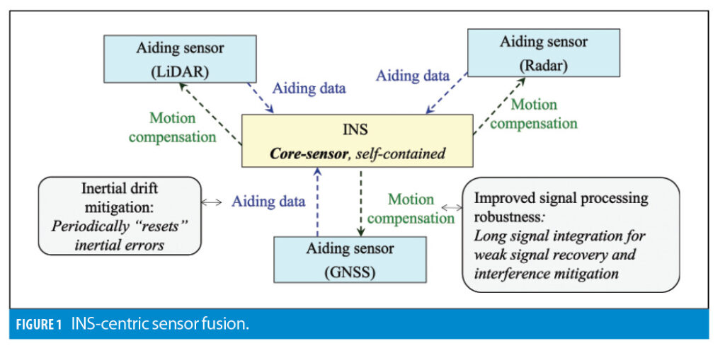
Figure 1 illustrates the sensor-fusion approach.
INS is used as a core sensor. It is augmented by aiding navigation data sources (such as GNSS or LiDAR) to mitigate the drift in inertial navigation outputs. Aiding sources generally rely on external observations or signals that may or may not be available. Therefore, they are treated as secondary sensors.
When available, aiding measurements are applied to reduce the drift in inertial navigation outputs. In turn, inertial data can be used to improve the robustness of an aiding sensor’s signal processing component, which is generally implemented in a form of motion compensation. For instance, INS-based motion compensation can be used to adjust replica signal parameters inside a GNSS receiver’s tracking loops to increase the signal accumulation interval, thus recovering weak signals and mitigating interference (jamming, spoofing and multipath). Another example is compensation of motion-induced distortions in EO imagery.
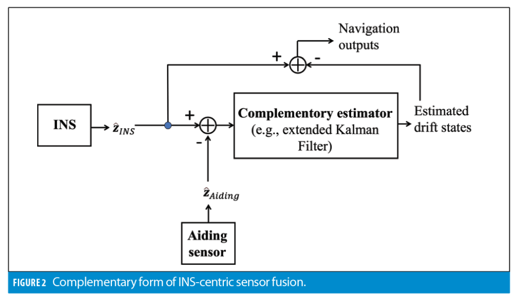
To mitigate inertial drift, sensor fusion uses the complementary estimation approach, which is illustrated in Figure 2.
As shown in Figure 2, differences between INS and aiding observations (zˆINS and zˆAiding) are applied to estimate inertial error states instead of navigation states. Error state estimates are then subtracted from the INS solution, thus providing the overall navigation output. Specific structure of the observation vector z depends on the integration mode.
The complementary formulation estimates INS error states rather than estimating full navigation states. As compared to the full-state formulation, the main benefit of complementary estimation is a significantly simplified modeling of state transition. Inertial errors are propagated over time instead of propagating navigation states themselves. In this case, the process noise is completely defined by stability of INS sensor biases, as well as sensor noise characteristics. On the contrary, modeling of actual motion generally needs to accommodate different motion segments (such as a straight flight versus a turn maneuver), which can require ad hoc tuning to optimize the performance. Moreover, propagation of navigation states through INS mechanization is a non-linear process.
In contrast, time propagation of inertial errors into navigation outputs can be efficiently linearized. As a result, complementary filters can generally rely on computationally efficient linear filtering techniques such as an extended Kalman filter (EKF) while reserving non-linear estimation approaches, such as particle filters and factor graphs, only to cases where aiding measurements are non-linear/non-Gaussian by nature, such as database aiding updates.
The integrated system operates recursively on the inertial update cycle. Every time a new measurement arrives from an inertial measurement unit (IMU), INS navigation computations are performed followed by the prediction update of the complementary filter. If an aiding navigation output becomes available after the previous IMU update, it is used to compute complementary filter observables and apply them for the estimation update. Otherwise, error estimates are assigned their predicted values and computations proceed to the next inertial update.
Integration Modes
The three main sensor fusion modes include loose coupling, tight coupling and deep coupling. They perform sensor fusion at the navigation solution level, measurement level and signal processing level, respectively. Their key features are:
Loose coupling
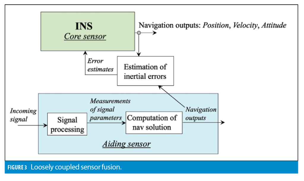
Figure 3 shows a high-level diagram of a loosely coupled system mechanization that fuses inertial and aiding data at the navigation solution level.
Aiding sensors generally include a signal processing part and a navigation solution part. The signal processing part receives navigation related signals and measures their parameters. For example, GNSS receiver tracking loops measure parameters (pseudoranges, Doppler frequency shift and carrier phase) of received GNSS signals. Another example is a LiDAR time-of-flight measurement that is directly related to the distance between the LiDAR and a reflecting object. Signal parameter measurements are then applied to compute the navigation solution. For example, GNSS pseudoranges are used to compute the GNSS receiver position. Changes in distances to reflecting stationary objects are exploited to compute the change in the LiDAR’s position.
Note the navigation solution can only be computed if a sufficient number of signal measurements is available. For example, at least four pseudoranges must be available to compute the GNSS-based position. At least two non-collinear lines must be extracted from an image of a two-dimensional (2D) LiDAR image to compute a 2D position. Depending on the aiding sensor, the observation vectors, zˆINS and zˆAiding can include, position, velocity, attitude and their combinations.
The loosely coupled approach operates at the navigation solution level and does not require any modifications to the aiding sensor. Yet, a key limitation of loosely coupled fusion is it cannot estimate INS error states unless a complete aiding solution is available. For instance, loosely coupled GNSS/INS cannot update inertial drift terms in an urban canyon when the GNSS position cannot be computed even though limited satellite measurements may still be available. As a result, useful aiding information is inherently lost.
Tight coupling
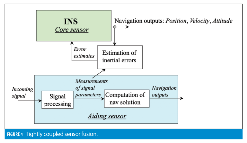
Tight coupling applies measurements of aiding signal parameters for the INS drift mitigation. As compared to loose coupling, the main benefit of tightly coupled systems is the ability to (partially) update INS error states even when insufficient aiding data are available to compute a full navigation solution, such as when less than four GNSS satellites are visible.
For such cases, a GNSS only position solution cannot be calculated. As a result, loosely coupled systems experience a complete GNSS outage. In contrast, the tightly coupled method can use limited GNSS measurements, thus enabling (partial) mitigation of the INS error drift. Another example of tight coupling is an EO-aided INS where landmark features are extracted from imagery data and then applied for the INS drift mitigation. When limited landmarks are present, and the system cannot compute an EO-based position update, individual feature measurements still enable INS drift mitigation within the tightly coupled architecture.
Figure 4 illustrates the tightly coupled approach.
For tight coupling, the INS error estimation generally has to be augmented with the estimation of aiding sensor errors. For example, GNSS receiver clock errors (bias and drift) are included into the system state vector for the GNSS/INS integration case. Image-aided inertial augments the system states with misalignment between INS and camera (or LiDAR) sensor frames.
Similarly to loose coupling, complementary estimation observables are formulated as differences between actual measurements and their INS-based estimates. To illustrate, for GNSS/INS, complementary pseudorange observations are formulated as differences between their INS estimates and GNSS measurements:

In Equation 1, is the geometrical range to the kth satellite. It is estimated using INS position solution, xˆINS, and satellite position vector,
:

where:

In Equation 2, x is the true position, δxINS is the INS position error, r(k) is the true range between the receiver and satellite k, (,) is the vector dot product, and | | is the Euclidian norm.
The GNSS pseudorange measurement model is:

where c is the speed of light, δtrcvr is the receiver clock bias, and ε is the pseudorange measurement error that includes thermal noise, multipath, atmospheric delays, and orbital errors.
From Equations 3 and 4, the complementary observation is formulated as:

The EKF is commonly applied to estimate INS error states and GNSS receiver clock states.
As mentioned previously, the main benefit of tight coupling is the ability to implement estimation updates even when limited signal measurements are available. As a drawback, it may require a firmware modification of the aiding sensor to enable access of its signal measurements, which are also referred to as raw measurements.
Deep coupling
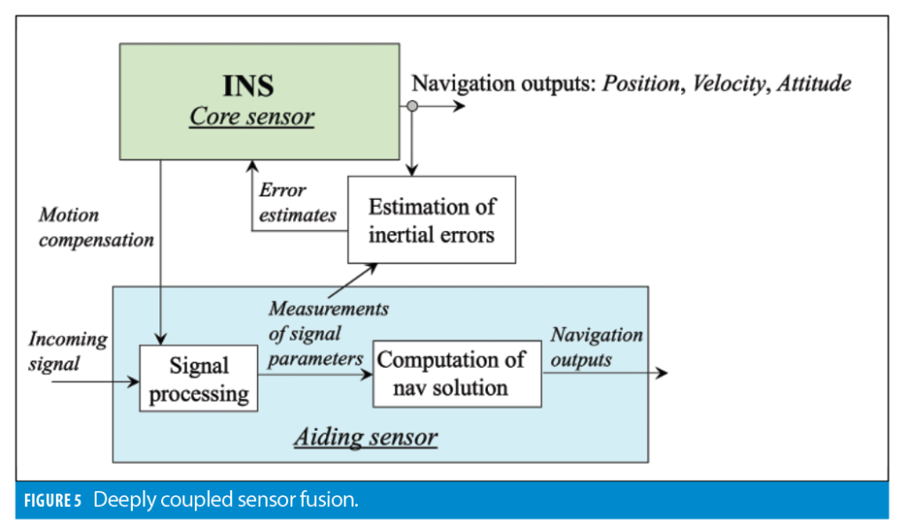
Deep coupling fuses inertial and aiding data at the signal processing stage. This approach keeps measurement-domain estimation of INS error states (as in tight coupling) and adds INS-based motion compensation to robustify the signal processing component of the aiding sensor. Figure 5 shows a high-level block diagram of the deeply coupled approach.
For GNSS/INS, various deeply integrated implementations, which are also referred to as ultra-tight coupling, have been reported in the literature. Both deep and ultra-tight systems are designed to improve the post-correlation signal to noise and interference ratio (SNIR). The distinction between deep and ultra-tight approaches can be somewhat vague. Ultra-tight coupled implementations generally maintain GNSS tracking loops and use inertial aiding to narrow their bandwidths. Deep integration operates directly with GNSS IQ samples. This is done by (i) processing IQ data with a combined pre-filter/Kalman filter scheme; or, (ii) explicitly accumulating IQ samples over an extended time interval (i.e. beyond the unaided receiver implementation).
Deep coupling maximizes the benefits of sensor fusion as it fuses inertial and aiding data at the earliest processing stage possible, thus eliminating any inherent information losses. However, it generally requires modification of the aiding sensor signal processing component. Yet, in some cases, these modifications still can be implemented via a firmware upgrade, for example, by providing access to high-frequency (1 kHz or similar) IQ outputs of GNSS correlators.
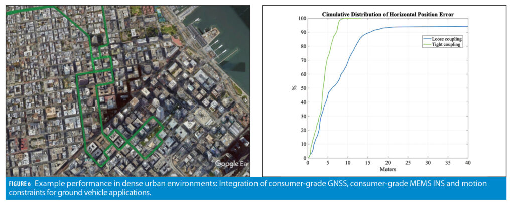
This section considers two example cases that illustrate benefits of INS-centric sensor fusion. The first example is the integration of GNSS and inertial for ground vehicle applications. Figure 6 shows example test results that compare loosely and tightly coupled system mechanizations. The system integrates a consumer-grade GNSS chipset, consumer-grade MEMS INS and vehicular motion constraints.
Cumulative error distribution results shown in Figure 6b clearly demonstrate the benefits of tight coupling over the loosely coupled approach. For example, the 90% bound of the horizontal position error is reduced from 15 meters to 6.5 meters, while the 95% error bound is reduced from 40 meters to 7.5 meters.
Example Benefits
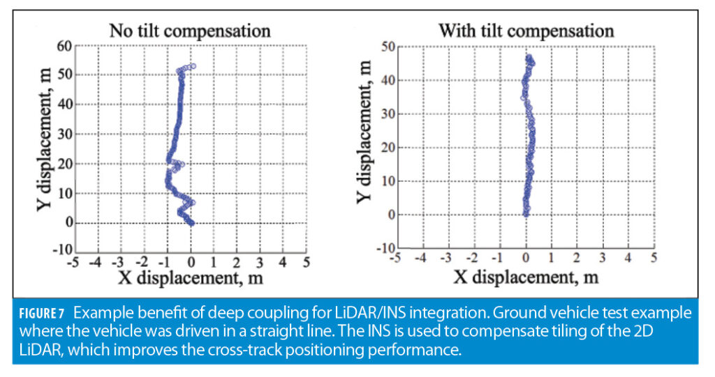
The second example illustrates the benefits of deep integration. Deep coupling for GNSS/INS (including weak signal recovery and interference mitigation) has been discussed by various research papers (including the first issue of The Inertialist column where we illustrated applications of deep integration for jamming and spoofing mitigation). In this section, example benefits are extended to non-GNSS aiding of inertial navigation.
Figure 7 shows example test results for a LiDAR-aided inertial. In this case, inertial data is fused with measurements of line features that are extracted from images of a 2D scanning LiDAR. The tightly coupled implementation assumes the LiDAR scanning plane remains horizontal, which leads to distortions in the cross-track direction as shown in the left-hand plot. Deep coupling applies inertial data to adjust LiDAR images for tilting, thus improving the cross-track performance as shown in the right-hand plot of Figure 7.
Conclusion
INS-centric sensor fusion uses self-contained inertial navigation as its core sensors and applies aiding data from other navigation aids to reduce drift in inertial navigation outputs. The complementary fusion enables seamless addition of aiding data (when and if available); PNT continuity in various environments; and robust, resilient state estimation with outlier mitigation (e.g., non-line-of-sight GNSS and SOOP multipath in urban environments) via INS-based statistical gating of aiding measurements.
The three main fusion strategies include loose, tight and deep coupling that subsequently increase the level of interaction between inertial and aiding sensors’ navigation and signal processing components. Progressing from loose to deep coupling improves the navigation accuracy and robustness. It may require modifications on the aiding sensor side, which in many cases can be accomplished via firmware upgrades.


