
In this second column we consider fundamental principles of inertial navigation that derive position, velocity and angular orientation from measurements of accelerometers and gyroscopes.
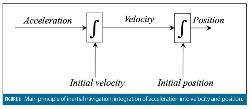
The key concept of inertial navigation originates from the first two laws of Newtonian physics. The first law states that an object will continue to move with a constant velocity unless disturbed by an external force. According to the second law, a non-zero net external force will result in an acceleration in the same direction with that force, and inversely proportional to the mass of the object. Hence, if we can measure the external force, it can be directly related to acceleration. Figure 1 shows how acceleration can be then integrated into velocity and position.
Clearly, integration requires initial conditions: i.e., initial velocity and position have to be determined. The initialization is commonly accomplished using external aids such as GNSS.
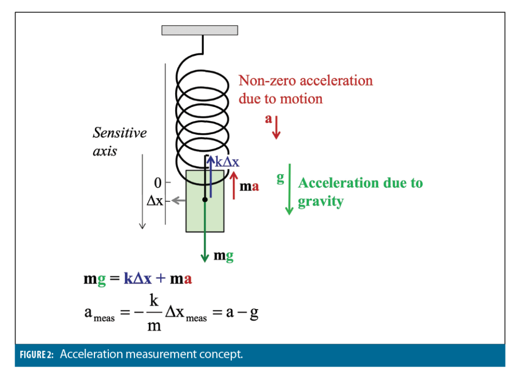
Acceleration is measured by accelerometers whose operational concept can be represented by a proof mass on a spring (Figure 2). An accelerometer measures projection of nongravitational acceleration (i.e., a difference between the acceleration due to motion and acceleration due to gravity) on its sensitive axis. In textbooks, this nongravitational acceleration is also referred to as specific force. To integrate accelerometer measurements into velocity and position, the INS first needs to relate orientation of sensors’ sensitive axes to a navigation frame of reference (where navigation outputs are computed). Second, gravitation acceleration needs to be added.
Gimballed and Strapdown
There are two approaches to relate measured projections of non-gravitational acceleration with the navigation frame. The first, referred to as gimballed, is to mechanically align accelerometer sensitive axes with the axes of navigation frame. For the second, referred to as strapdown, accelerometers are rigidly attached to the (rotating) body frame and the angular alignment is performed computationally. The gimbaled approach allows for a very precise angular alignment. However, it results in larger size, higher cost and reduced reliability (increased mean time before failure) of inertial navigation as compared to strapdown implementations. Hence, most modern inertial systems utilize a strapdown approach wherein sensor’s sensitive axes are rigidly attached to the body frame and stabilized computationally rather than mechanically. Here, gyroscopes measure angular rates, which are then applied to compute relative attitude between body and navigation frames. Attitude estimates then computationally transform components of the non-gravitational acceleration vector from body into navigation frame.
In addition, Newton’s laws are valid only in a non-rotating inertial frame. For the majority of navigation applications, navigation solution needs to be determined relative to an Earth-related frame of reference such as a local-level East, North Up (ENU) frame. These rotating frames are non-inertial by nature. Hence, compensation of non-inertial effects has to be added to the INS navigation mechanization.
System Components
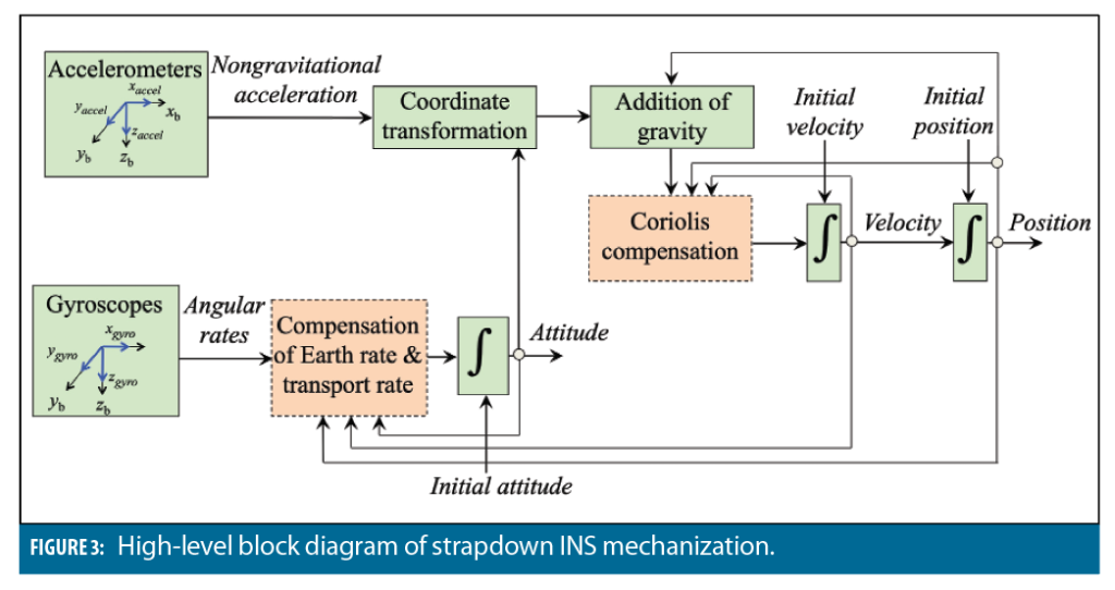
Summarizing, the main principle of inertial navigation (illustrated in Figure 1) needs to be extended to include (i) attitude stabilization, (ii) addition of gravity; and (iii) compensation of non-inertial effects. Figure 3 shows a respective high-level diagram of strapdown INS mechanization.
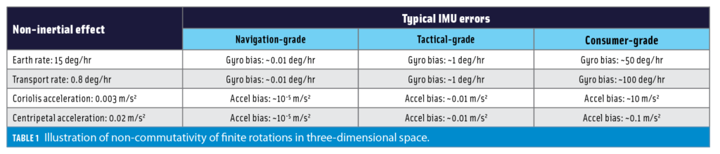
In Figure 3, solid lines indicate components that are required for any type of INS. System components with dotted-lines can be omitted by some inertial implementations, particularly, when lower-grade MEMS sensors are used. These components are related to compensation of non-inertial effects, including (1) the Earth rate (rotation of the Earth), (2) the transport rate (rotation of the local-level frame due to platform’s motion along the Earth surface), (3) Coriolis acceleration and (4) centripetal acceleration (which is often incorporated into addition of gravity). Their compensation requires knowledge of velocity and position states, as well as angular orientation. Hence, a feedback from velocity, position and attitude computations is included in Figure 4. Compensation of non-inertial effect is a more advanced INS concept that can be found in textbooks on inertial navigation and is not further considered as a part of this description of inertial fundamentals. In addition, for lower-grade IMUs, non-inertial effects stay below the level of sensor errors (biases and noise). Table 1 shows this with numerical estimates for an example case where a ground vehicle is moving with a speed of 60 mph at a 45 deg Northern latitude. The table demonstrates that higher-grade inertial systems (tactical and navigation grade) must compensate for non-inertial effects; these can be considered second-order, excluded from INS mechanization, when consumer-grade IMUs are used.
Angular Orientation
As shown in Figure 3, gyro angular rates are integrated into angular orientation for computational alignment of accelerometer sensitive axes with the navigation frame. Angular orientation is commonly represented by Euler angles, quaternions and direction cosine matrix (DCM). There is no one particular attitude parametrization that would provide substantial advantages over others (in terms of computational savings or reduced error propagation) and all three methods can be used interchangeably. We will apply DCM to represent INS attitude due to its intuitive use for coordinate transformation. The notation is for the DCM that corresponds to the coordinate transformation from body (b) into navigation (N) frame.
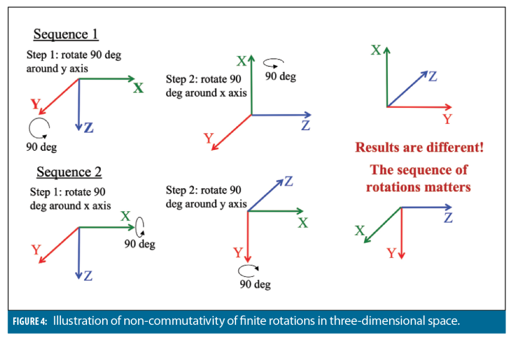
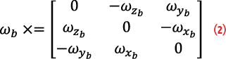
Unfortunately, finite rotations do not commute in three dimensions (Figure 4). This complicates INS attitude updates. Gyro angular rates cannot be simply integrated into rotation angles around x, y and z axes and then converted into attitude, since the sequence of rotations matters. Fortunately, infinitesimally small rotations commute, producing an attitude differential equation. For the case of DCM, this equation is:

where is the skew-symmetric matrix comprised of body-frame angular rates:
Equation (1) is an exact continuous-time relationship between the DCM and angular rates. Its exact discrete-time solution can be obtained for a case where orientation of the angular rate vector stays constant between consecutive IMU updates:

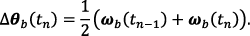
where is the matrix exponential function, and is the skew symmetric matrix of body-frame angular increments over the IMU update interval. Some IMUs output gyro measurements in the form of angular increments (delta Thetas), which can be directly used for DCM updates. Otherwise, gyro rates can be numerically integrated into angular increments, using, for example, a trapezoidal rule:
Equation (3) is the exact DCM solution, assuming that angular rate vector does not change orientation between consecutive IMU updates (the vector’s absolute value can change). When this does not hold, computational errors are introduced, referred to as coning errors, to be considered in future columns.
Similar to integration of acceleration into velocity and position, INS attitude requires initialization: i.e., initial value of the DCM, needs to be estimated. It can be then propagated recursively over time using equation (3). Initial attitude is estimated based on vectors whose components are known in body and navigation frames: body frame is computationally rotated such that body and navigation frame components of these vectors are aligned with each other.
When at least two non-collinear vectors are available, a unique rotation exists that defines initial value of the DCM. Most commonly, gravity and Earth rate vectors are applied for the initial alignment. Their body-frame components are measured by accelerometers and gyros, respectively, when the IMU is stationary; while navigation-frame components are obtained using GNSS position estimate (gravity is derived from a model and Earth-rate is projected into the ENU frame for a given location).
However, for lower-grade IMUs, Earth rate (15 deg/hr) stays below gyro errors and cannot be measured reliably. In this case, the following initialization method can be used. First, angular orientation is partially aligned using gravitational acceleration while the platform is stationary. Next, a straight motion segment is exercised during which velocity vector is applied to complete the alignment procedure. Navigation frame components of velocity are estimated from GNSS data. Body-frame components are defined from a motion model: for example, assuming that velocity is aligned with the vehicle’s forward axis.
Figure 3 shows angular orientation used to transform body-frame nongravitational acceleration into navigation frame:

Coordinate transformation is followed by the addition of gravity:

Gravity addition uses a model of gravitational acceleration vector. The simplest model is to assume that this vector is pointer downward and its absolute value is equal to 9.8 m/s2. This model’s accuracy is sufficient for lower-grade inertial systems. However, more accurate gravitational models are required for higher-grade INS. In this case, gravitational model represents direction and magnitude of gravity as a function of position.
Finally, navigation-frame acceleration is numerically integrated into velocity and position outputs:


Note that more advanced integration schemes (i.e., quadratic or higher-order) can be used to reduce numerical errors in high dynamic-motion environment.
Complete Algorithm
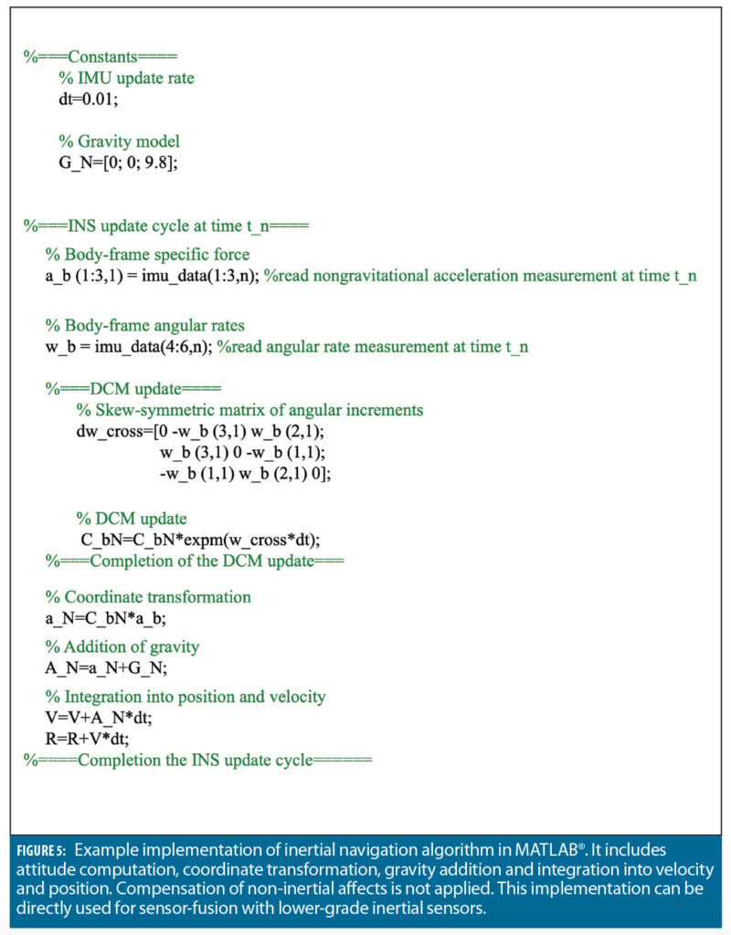
To summarize basic INS mechanization, Figure 5 shows a MATLAB implementation of inertial algorithm that follows main computational steps.
INS implementation in Figure 5 does not include compensation of non-inertial effects. As discussed previously, these effects stay below IMU sensor errors for lower-grade inertial systems (such as consumer-grade MEMS). As a result, the algorithm in Figure 5 has been successfully used by various INS-centric sensor-fusion systems, such as for example tightly and deeply coupled GNSS/INS mechanizations that were discussed in the first issue of the Inertialist column.


