 Figure 1
The downloadable PDF (above) contains bonus material not available in the print edition. Appendices and other information on this subject is available at the bottom of the page.
The current version of the master GPS Interface Specification document (IS-GPS-200 Rev D March 2006) contains a new dual-frequency ionosphere correction algorithm that is to be used with the modernized GPS space vehicles (SVs) and their next-generation modernized GPS signals.
The Block IIR-M satellites add the new L2C, L1M, and L2M signals on the existing L-band carriers. The Block IIF will also transmit these signals as well as a new L5 signal on the recently established L5 carrier.
Signals/ranging/modulation codes all refer to the various GPS broadcast waveforms that can be present on the L1, L2, or L5 carriers. These codes perform three functions: code division multiple access (CDMA), processing/anti-jam gain, and indication of transmission time by providing each chip a unique time-tag.
The “new” algorithm, which we refer to as “the modernized ionosphere-free pseudorange algorithm,” contains a mix of new parameters, inter-signal corrections (ISCs), and the legacy scaled group delay differential parameter TGD. This article describes why a new algorithm is needed, and how the new and old parameters are combined.
With the U.S. Air Force set to begin broadcasting this fall the first of the new CNAV navigation messages on the L2 civil signal transmitted by the Block IIR-M satellites, an understanding of these issues will be important for GPS receiver designers, GNSS signal simulator manufacturers, and end users who require high-precision results from their GPS equipment.
In our presentation, we will first derive the new algorithm by using IS-GPS-200’s definition of delay error to model the GPS satellite equipment delays. Then, working through the various paragraphs on how to perform single- and dual-frequency corrections, we can reconstruct the new equations by analyzing the modernized SV model.
Having this modernized model allows one to also derive new results, such as a modernized version of the popular alternative ionosphere correction algorithm — the ionosphere pseudorange difference algorithm and understand why the new algorithm offers a more accurate correction.
Background
Terrestrial users can experience between 3 to 30 meters of ionospheric ranging error due to the effects of phenomena encountered by signals propagating through the atmosphere. At L-band frequencies for a nominal ionosphere, the measured ionosphere range is reasonably modeled as an error that is inversely proportional to the square of the carrier frequency.
If no other significant frequency-dependent errors exist, two ranging measurements on different L-band carrier frequencies allow the ionosphere error to be eliminated.
In general, until now only Department of Defense (DoD) receivers that track both the L1 P(Y) and the L2 P(Y) signals could make such a correction. (Some civilian receivers can track the DoD P(Y) code without a crypto key when the signal to noise ratio is sufficiently “high.”)
With modernized GPS, however, civilian users will finally have access to a second frequency, the new L2C and/or L5 signals. For DoD users, the new L1M and L2M military signals will provide better cryptography as well as improved accuracy.
Moreover, because a pair of M codes will reside on different carriers, dual-frequency ionosphere corrections capability can be maintained on modernized GPS military user equipment.
Because we cannot precisely eliminate small variations in SV equipment delays among the various signal paths within the satellite, these new signals — as well as the legacy signals — don’t exactly emerge from the satellite antenna at the same time or from the same location.
If not accounted for, these delay offsets would produce GPS navigation fix errors for dual- and single-frequency users.
Consequently, IS-GPS-200 provides one ISC for each signal on each L-band. So, a Block IIRM SV with L1 CA, L1P(Y), L1M, L2C, L2P(Y), and L2M, has six ISCs. A GPS follow-on Block IIF satellite that also includes L5I and L5Q (in phase and in quadrature signals, respectively) will have two additional ISCs. The legacy TGD parameter is really the ISC parameter for L2P(Y) scaled by a constant, which we will discuss later.
We will use the following subscript notation when a pair of L-band measurements is being discussed: Li,x will denote one carrier frequency with signal x, and Lj,z will be used for the second L-band carrier frequency and the signals on that carrier. So for L1, Li=L1, and x=CA, P(Y), or M codes. For L2, Lj=L2, and z=L2C, P(Y), or M. For L5, Lj=L5, and z=L5I or L5Q.
In all of the dual frequency correction algorithms, IS-GPS-200 and IS-GPS-705 use the symbol γij to represent the ratio of (fLi/fLj)2 of the L-band carrier frequencies squared. If γ is not subscripted, one can assume that it is γ12.
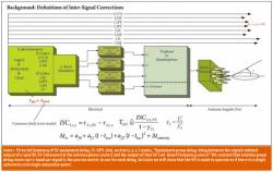
To understand where the small SV equipment–delay errors come from, consider putting a picture to the words in paragraph 3.3.1.7 of IS-GPS-200 in order to build up a model of the modernized SV as shown in Figure 1 (above right).
According to paragraph 3.3.1.7, the SV-equipment group delay for each signal is the amount of time it takes the signal to start out from the common clock, travel through each code generator, modulator, transmitter, tri- or quadraplexor, and finally emerge from the satellite’s antenna. Thus, the total delay consists of an electrical portion and an antenna portion.
Note that the SV antenna is effectively a two-element array, made up of an inner-ring that produces a broader beam and an outer ring that produces a narrower beam. As discussed in the articles by C. Choi and by G. Mader and F. Czopek listed in the Additional Resources section near the end of this article, the two rings are effectively phased 180 degrees apart so that the narrower beam is subtracted from the wider beam.
As a result, the power across the surface of the Earth over the 13-degree half angle of the transmitted signal is approximately constant.
Because the SV antenna is an array, it can have gain, phase, and group delay variations across the beam, although for a properly designed antenna array, any angular variations of delay and phase would be small compared to the total signal-in-space (SIS) error budget.
Choi’s article notes the distinct locations of the phase centers for each L-band — all signals within an L-band sharing the same phase center, but it does not discuss the group delay characteristics of the SV antenna, nor does it discuss the possibility that each L-band signal may have its own distinct group delay center.
As noted earlier, ISCLi,x is the difference of the transit delay through the SV (including antenna) for L1P(Y) minus the transit delay for the xth or zth signal on the Li or Lj carrier.
(It is important to point out that the ISC values, one for each signal, are not affected by the common clock error modeled by a second order polynomial with the coefficients af0, af1, and af2 broadcast in subframe 1, as noted in the center of Figure 1, because this error is common to all signals and won’t contribute to delay differences.)
The ISC values may age with time or change when redundant components are swapped in as the satellite ages. Each satellite has its own set of ISC values. The legacy parameter TGD is really ISCL2P(Y) scaled by (1-γ).
The ISCs for civil users are broadcast in Message #30 of the CNAV dataset, and the M-code ISCs will be present in the MNAV dataset. The values are based on contractor-measured data. For TGD, on-orbit data is also used, as discussed in the article by B. Wilson et alia listed in Additional Resources.
Problem and Simplified Solution
In this section, we mathematically state our problem and provide a simplified derivation of the legacy versus modernized ionosphere-free pseudorange algorithms by building up a pseudorange error model that properly accounts for SV equipment delays consistent with the IS-GPS-200 ISC parameters, but without delving into the detailed IS-GPS-200 notation.
We should note that, strictly speaking, IS-GPS-200 defines the ISCs in terms of time-tag differences, not delay differences, and it takes a substantial amount of effort and verbiage to prove that the delay notation we use is equivalent to the time-tag notation used in reference 1.
Also of interest is the fact that, historically, IS-GPS-200 was written for engineers who were building entire GPS receivers; thus, many of the compensation algorithms are stated in terms of the delay lock loop’s code phase read-out of the time of transmission as measured by the receiver. Only later is the final pseudorange formed as the user time minus time of transmission scaled by the speed of light, c.
For our full derivation of the new algorithm with all of the exhaustive details, readers can download an extended version of this article using the PDF link at the top of this story.
Although IS-GPS-200 can be tedious to read, a tremendous number of insights can be gleamed from it. (As an aside, it would be nice if a team of authors could write a companion document to IS-GPS-200 that describes why certain decisions were made, and to provide derivations, so that valuable knowledge will not be lost as people retire.)
For the complete, extended version of this story, including figures, equations, and the following topics, please download the PDF of the article, above.
- Problem Statement
- In Search of the Modernized Ionosphere-Free Pseudorange Equation
- Simplified IS-GPS-200 Modernized Ionosphere Algorithm Derivations
- Further Steps in Deriving the Ionosphere Correction Algorithm
- Final Approach to the Equation
- Simplified Alternative Algorithm Derivations
- Interpreting the Modernized SV Model and Ionosphere Correction Equations
- GPS Constellation Simulators and Receivers
- Conclusions and Future Work
Acknowlegments
The authors would like to thank Ken Jones of Spirent, Soon Yi, at the Aerospace Corporation, G. Okerson at SRI International, and R. Greenspan and S. Buckley at C. S. Draper Laboratory for help with reviewing this article. We would also like to thank USAF Capt. Valerie Avila for her encouragement over the last two years. Finally, Avram Tetewsky would like to acknowledge J. Furze of Draper Laboratory, a mentor and unique task leader, for “asking me the right questions that helped me truly understand GPS.”
Additional Resources
[1] Choi, C., “Phase Centers of GPS IIF Modernization L-Band Antenna,” Proceedings of ION GPS 2002, 24-27 September 24–27, 2002, Portland, Oregon, USA
[2] IEEE Antenna Model, IEEE Std 145-1993 (R2004), 1993
[3] IS-GPS-200 March 2006 Rev D (also in 2004 version)
a) page 17, paragraph 3.3.1.7, defining equipment group delay from frequency source to antenna phase center, but not defining antenna phase center to be for all L-bands or only one L-band.
b) page 88, 20.3.3.3.3.1 — User Algorithm for SV Clock Correction. Of particular interest: “The polynomial defined in the following allows the user to determine the effective SV PRN code phase offset referenced to the phase center of the antennas . . . ,” but not indicating if it is the L1, L2, or L5 phase center.
c) page 90, 20.3.3.3.3.2. L1 – L2 correction and the definition of TGD
d) page 99, 20.3.3.4.3.2. Parameter sensitivity of antenna phase center
e) page 169, 30.3.3.3.1.1.1. Inter-Signal Group Delay Differential Correction, and page 170, 30.3.3.3.1.1.2. L1/L2 ionospheric correction for L1C/A and L2C SV manufacturers will supply these values, definitions of ISC and equipment delay.
f) Definition of the inter-signal corrections (ISCs)
[4] IS-GPS-705, 20.3.3.3.2.5 has the L1/L5 modernized dual-frequency correction. Kaplan, E., and C. Hegarty, “Understanding GPS Principles and Applications”, Second Edition, Artech House, 2006, (page 313, 7.23 and page 309 for group delay versus phase delay)
[5] Kraus, J., Antennas, Second Edition, McGraw Hill, 1988
[6] Mader, G., and F. Czopek, GPS World, “The Block IIA Satellite, Calibrating Antenna Phase Centers,” May 2002
[7] Misra, P., and P. Enge, GPS Signals, Measurements, and Performance, Second Edition, Ganga-Jamuna Press, page 166, 5.30, and pages 159–160 for group delay versus phase delay.
[8] Murphy, T., and M. Harris, P. Geren, T. Pankaskie, “GPS Antenna Group Delay Variations Induced Errors in a GNSS Based Precision Approach and Landing System,” Proceedings of ION-GNSS 2007, September 25–28, 2007, Forth Worth, Texas, USA
[9] U.S. Air Force, “The Precise Positioning Service (PPS) Performance Standard,” <http://gps.afspc.af.mil/gpsoc/> and <http://gps.afspc.af.mil/gpsoc/gps_documentation.htm>, <http://gps.afspc.af.mil/gpsoc/documents/PPS_PS_Signed_Final_23_Feb_07.pdf>
[10] Van Graas, F., and C. Bartone and T. Arthur, “GPS Antenna Phase and Group Delay Corrections,” Proceedings of the ION National Technical Meeting 2004, January 26-28, 2004, San Diego, California, USA
[11] Wilson, B., and C. Yinger, W. Feess, Capt. C. Shank, “New and Improved: The Broadcast Intefrequency Biases,” GPS World, June 1999


