
Learning GNSS positioning corrections for smartphones using Graph Convolution Neural Networks.
ADYASHA MOHANTY AND GRACE GAO, STANFORD UNIVERSITY
High-precision positioning with smartphones could bring in-demand technologies to users around the world. It would enable applications such as lane-level accuracy for road users and autonomous cars, precise mapping, indoor positioning, and improved localization in augmented reality-based gaming environments. In the last few years, raw GNSS measurements from smartphone receivers have become more publicly accessible, as demonstrated by the release of the Android GNSS application program in 2016 [1] and the Google open datasets in 2020 [2]. More recently, Google launched the Google Smartphone Decimeter Challenge (GSDC) [2] to invest in the development of novel technologies that can obtain high-precision positioning from smartphone measurements.
The current challenge with smartphone receivers is they can only offer 3 to 5 meters of positioning accuracy under good multipath conditions and over 10 m accuracy under harsh multipath environments. Due to limitations in GNSS chipset, size and hardware cost, GNSS measurements from smartphones have lower signal levels and higher noise compared to commercial receivers [3,4].
However, new opportunities have emerged that can be leveraged to design novel positioning algorithms. For example, with the advent of the new Android API, raw GNSS measurements have become more publicly accessible, which has encouraged the development of new tools and software for processing these datasets. We also have access to multi-frequency and multi-constellation measurements that provide redundancy while navigating in dense urban canyons where GNSS measurements from a single frequency/constellation can be sparse. Lastly, we also have the capability to use more precise measurements, such as carrier phase measurements, for providing decimeter-level accuracy.
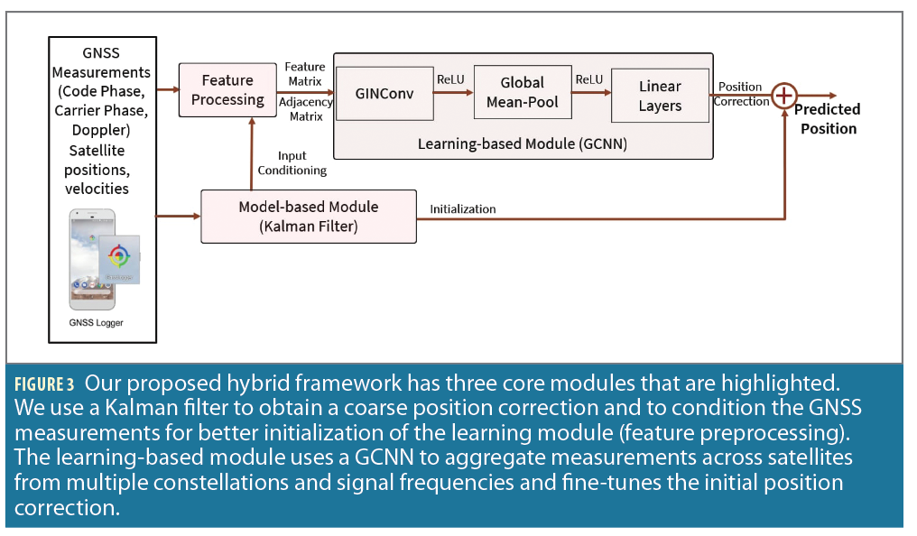
In this article, we propose a hybrid framework that combines the benefits of both learning-based and model-based methods to learn position corrections from smartphone GNSS measurements. For the learning-based approach, we use a Graph Convolutional Neural Network (GCNN) that predicts a position correction given an initial coarse receiver position. To overcome the sensitivity of the GCNN to the inputs, we use a model-based approach, a Kalman filter, to predict an initial position and to condition the input measurements to the graph. The GCNN then predicts a finer position correction by applying convolution operations to the input graph. Given the success of Factor Graphs in winning both the 2020 and the 2021 GSDC challenge [5], GCNN forms our design choice for the learning-based approach because it can learn such a graph with satellite positions as nodes and preconditioned inputs from the Kalman filter. It is also capable of handling varying satellite visibility in urban environments via an unordered structure of nodes and is able to model measurements from multiple constellations and multiple signal frequencies.
Given a graph structure that is derived from known properties of GNSS measurements and the Kalman filter solution, the GCNN performs inference in an end-to-end manner where the graph structure helps propagate information among neighboring nodes [6].
Proposed Algorithm
Background on GCNN
Traditionally, neural networks have shown high predictive power on learning tasks that need fixed-size and regularly-structured inputs. However, graph neural networks can operate on vector data structures such as a graph and make more informed predictions by using features from the graph nodes. A subset of graph neural networks, GCNN [5] offers the same advantages with the extended capability of performing convolutions on arbitrary graphs. Even though ordinary convolutions are not node-invariant, GCNNs still retain the permutation-invariance properties of a graph neural network. This property indicates the function the graph learns is independent of the rows and columns in the adjacency matrix. It also implies that changing the order of the inputs (or the nodes in the graph) would not affect the graph-level prediction. This feature makes GCNN suitable to model the varying number of GNSS satellites at every time step.
A GCNN as shown in Figure 1 takes as inputs a connected graph G = (V,E) where V represents the nodes, E represents the edges [6].
The graph also takes additional inputs. The first input is an adjacency matrix representation A that depicts the connection of each node to its neighboring nodes. In A, an element has a value of 1 of two nodes i and j are connected. The second input to the graph is a feature matrix X that describes the graph signal on every node. The matrix X has n rows and contains d signals of the graph and represents all the node features stacked together. Every layer of the neural network is then written as a non-linear function as follows:

Where Hl and H(l + 1) represent the output from the hidden layers of the network and the function g(.) is learned by the GCNN.
More details about the formulation of the propagation rule for each convolution layer of the GCNN can be found in [6].
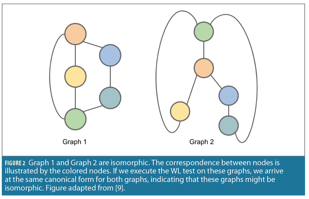
The WL isomorphism test [8] is a popular method that checks the representative power of different GCNNs. More specifically, it checks for graph isomorphism, i.e., two graphs are considered isomorphic if there is a mapping between the nodes of the graphs that preserves node adjacencies as illustrated in Figure 2. The WL test produces a canonical form for each graph. If the canonical forms of two graphs are not equivalent, then the graphs are not isomorphic. In a message passing layer within a GCNN, the features of each node are updated by aggregating the features of the node’s neighbors. The choice of the convolution and aggregation layers are important because only certain choices of GCNN satisfy the WL test and are thus able to learn different graph structures.

Kalman Filter Initialization
To mitigate the sensitivity of the network to initial inputs, we provide an initial position to the network that is a coarse estimate of the receiver’s true position. We chose a Kalman filter as our model-based approach because it uses the temporal history of GNSS measurements, converges quickly and is computationally efficient.
We first select GNSS measurements based on CN0, satellite elevation and carrier error values and then compute the receiver’s position using the Kalman filter.
Feature Preprocessing
We preprocess the GNSS measurements using the following steps:
1. We group all the measurements into different constellations and signal types.
2. We eliminate inter-system and inter-frequency biases, clock biases, tropospheric and ionospheric errors from the code phase measurements.
3. We apply carrier smoothing to the code phase measurements by using the ADR measurements. In the event of a cycle slip, we use Doppler values for smoothing the code phase measurements. Note the presence of a cycle slip is indicated by a bitwise operation that is recorded from the receiver.
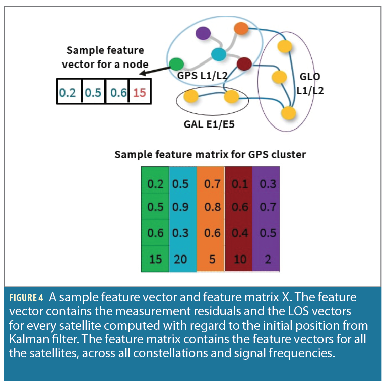
Using the satellite grouping (Step 1) and the smoothed code phase measurements (Step 3), we construct feature vectors for every satellite. Because the choice of features is a design choice, as a proof of concept, we use simple features for the GCNN, such as LOS vectors and measurement residuals. Given the initial position estimate from the Kalman filter and satellite positions, we compute the LOS vector and measurement residuals for each satellite.
GCNN: In the graph, we represent each node using the satellite position. Given the feature vectors for every node, we can form the feature matrix for the entire graph. A sample feature vector and feature matrix are illustrated in Figure 4.
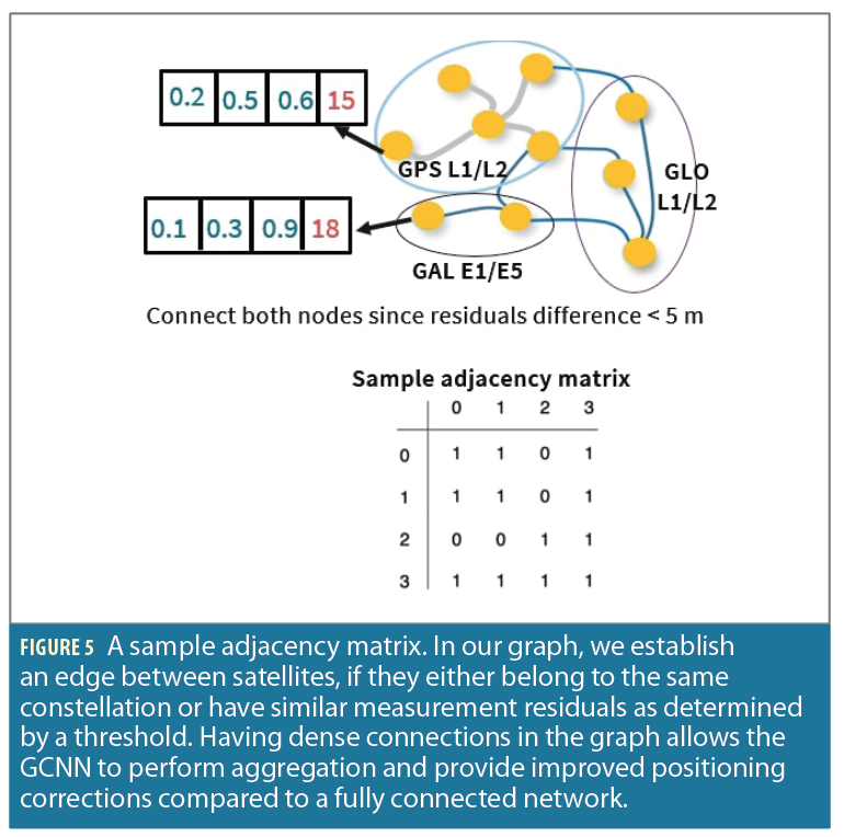
For creating the adjacency matrix, we establish edge connections between satellites that belong to the same constellation as well as connections between satellites from different constellations if their node features have similar measurement residuals. A sample adjacency matrix is illustrated in Figure 5.
Convolution Layers and Prediction
There are many available choices of convolution layers. For our work, we chose Graph Isomorphism Network (GIN) Convolution [10] layers because these layers satisfy the WL graph
isomorphism test and achieve maximum discriminative power among all other graph neural networks.
We learn an aggregation function over the features associated with each node in the graph, akin to the concept of an attention module, as explored in [11]. There are multiple choices for the aggregator function, such as the mean aggregator, LSTM aggregator and pooling aggregator. For this work, we perform a mean pooling across all the graph nodes because our final output is a graph-level prediction instead of a node-level prediction. Pooling instantiates message passing among different nodes of the network, allowing the neighboring nodes to update their features and weights concurrently. Pooling also reduces the spatial resolution of the graph for subsequent layers. Post-aggregation, we pass the updated features at every node through a series of fully connected linear layers that increase graph expressivity and improve our final prediction.
For inferring the position correction, we train the entire graph using a standard Euclidean loss function that is constructed from the estimated positioning correction and the true correction obtained from ground truth. Note we can construct this loss function only at training time because we do not have access to the true correction during inference.
Experiments and Setup
We test our proposed algorithm on the GSDC 2021 datasets [2] that contain GNSS code phase, ADR, Doppler measurements, and ground truth from a GNSS-INS integrated SPAN system.
Baselines and metrics
We compare our proposed algorithm against two baselines: A weighted-least squares solution that is a snapshot
positioning method and a Kalman filter solution, which is a temporal method. We tune both baselines using Bayesian hyperparameter optimization for achieving maximum performance on the test datasets. We use quantitative metrics such as the mean, median, maximum and minimum horizontal positioning error. We also study the distribution of positioning error for the baselines and our algorithm. For qualitative results, we compare the predicted trajectory from all the algorithms with regard to ground truth trajectory.
Evaluation and Key Parameters
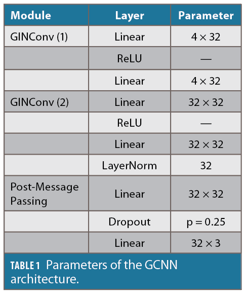
We split the GSDC datasets into 81 training datasets and 17 test datasets. Some of the test datasets contain data collected in cities previously and separately from the training datasets. This was a design choice to stress test our proposed approach. We leverage the publicly available tool Pytorch Geometric [11] to design, train and test the GCNN module of our framework. We train the GCNN for 100 epochs using an MSE loss function and Adam optimizer [12]. We performed training across multiple hardware platforms such as Kaggle, Google Colab and Amazon AWS using GPU and TPU accelerators for faster training. The network architecture and the number of parameters in each layer are shown in Table 1.
Results
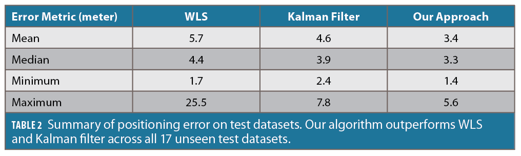
We analyze the horizontal positioning error across all 17 unseen test datasets first. As shown in Table 2, our algorithm outperforms both the snapshot method (WLS) and the temporal method (Kalman filter) for each metric. Our approach leads to the lowest mean, median, minimum and maximum error on all 17 datasets.
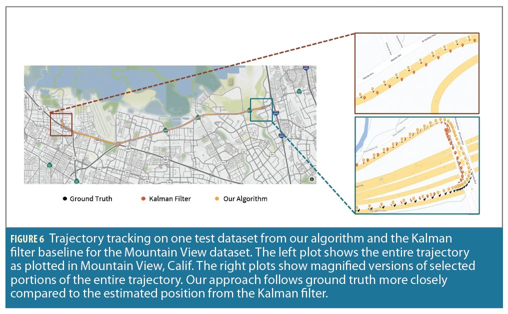
We then show qualitative results via sample trajectory plots in Figure 6 that are generated by plotting the position predictions from our algorithm and the Kalman filter baseline for the Mountain View
dataset. The figure indicates our algorithm is able to track the ground truth trajectory closely while showing improvement in regions that are depicted by the magnified plots. In these regions, we observe the predictions from the Kalman filter baseline show some deviations. However, the GCNN module is able to fine-tune the correction and compensate for the deviations leading to improved results from our algorithm.
For the next set of results, we only show results from the Kalman filter baseline for easier comparison because the predicted positions from the WLS baseline always have the highest errors. We study the distribution of the horizontal positioning error on selected test datasets. For this purpose, we consider both the Mountain View dataset and an additional dataset collected in Los Angeles.
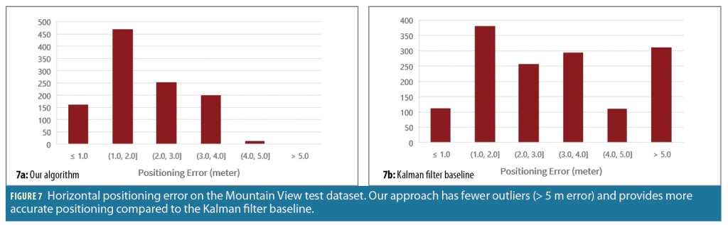
Figure 7 shows the error distribution from our evaluation of the Mountain View dataset. We observe that, compared to the Kalman filter baseline, our algorithm has few outliers defined to be positioning errors > 5 m. Additionally, our algorithm provides more accurate positioning compared to the Kalman filter because our error distribution has higher instances of error in the range of 0 to 3 m.
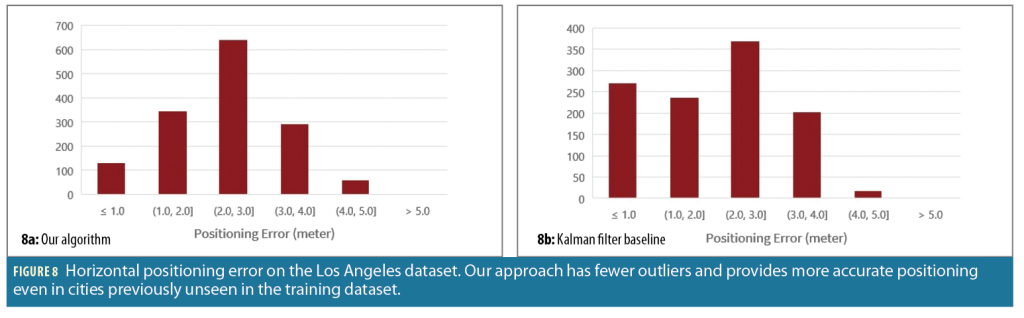
We also analyze the error distribution on the LA dataset as shown in Figure 8. Similar to the Mountain View test dataset, our approach provides positioning with fewer outliers than the Kalman filter baseline and shows improved positioning with most errors in the range of 1 to 3 m.
Conclusions
We designed a hybrid approach for inferring position corrections from smartphone GNSS measurements using a Graph Convolutional Neural Network (GCNN) and initial position estimate from a Kalman filter. For the GCNN, we created features using measurement residuals and LOS vectors from multiple GNSS constellations and multiple signal frequencies after applying carrier smoothing. The GCNN performed aggregation across all available satellites and learned the position correction in an end-to-end manner. We evaluated our approach on real-world datasets collected in urban environments. Our approach demonstrated improved positioning accuracy and error distribution when compared against model-based approaches such as WLS and Kalman filter. Thus, our approach is a promising fusion of existing model-based and data-driven methods for achieving high smartphone positioning accuracies in urban environments.
Acknowledgements
We would like to thank Google for releasing the smartphone datasets for 2020 and 2021. We would also like to acknowledge Zach Witzel and Nikhil Raghuraman for their help with debugging and Adam Dai and Daniel Neamati for reviewing the paper.
Lastly, we would like to thank members of the Stanford NAVLab for their insightful discussions and feedback.
References
[1] Humphreys, T. E., Murrian, M., Diggelen, F. V., Podshivalov, S., & Pesyna, K. M. (2016, 04). On the
feasibility of cm-accurate positioning via a smartphone’s antenna and GNSS chip. , 232-242.
(https://doi.org/10.1109/plans.2016.7479707)
[2] Fu, G. M., Khider, M., & van Diggelen, F. (2020, 09). Android raw GNSS measurement datasets for
precise positioning. In Proceedings of the 33rd international technical meeting of the satellite division of
the institute of navigation (p. 1925-1937). Virtual. (https://doi.org/10.33012/2020.17628)
[3] Guangcai, L., & Jianghui, G. (2019, 07). Characteristics of raw multi-GNSS measurement error from
Google Android smart devices. GPS Solutions, 23, 1-16. (https://doi.org/10.1007/s10291-019-0885-4)
[4] Zhang, K., Jiao, F., & Li, J. (2018, 05). The assessment of GNSS measurements from android
smartphones. In Proceedings of the china satellite navigation conference (p. 147-157). Harbin, China.
(https://doi.org/10.1007/978-981-13-0029-5 14)
[5] Suzuki, T. (2021, 09). First place award winner of the smartphone decimeter challenge: Global
optimization of position and velocity by factor graph optimization. In Proceedings of the 34th
international technical meeting of the satellite division of the institute of navigation (p. 2974 – 2985). St.
Louis, Missouri. (https://doi.org/10.33012/2021.18109)
[6] Kipf, T. N., & Welling, M. (2017). Semi-supervised classification with graph convolutional networks. In
Poster presentation at the international conference on learning representations (iclr). Toulon, France.
(https://doi.org/10.48550/arXiv.1609.02907)
[7] Jian, D., Shi, J., Kar, S., & Moura, J. (2018, 06). On graph convolution for graph CNNS. In Ieee data
science workshop (p. 1-5). Lausanne, Switzerland. (https://doi.org/10.1109/DSW.2018.8439904)
[8] Weisfehler, B., & Leman, A. (1968). The reduction of a graph to canonical form and the algebra which
appears therein. In Nauchno-technicheskaya informatsia (Vol. 9).
[9] Beiber, D. (2019, 05). Weisfeiler-Lehman isomorphism test. In Online blog post.
(https://davidbieber.com/post/2019-05-10-weisfeiler-lehman-isomorphism-test/)
[10] Xu, K., Hu, W., Leskovec, J., & Jegelka, S. (2019, 05). How powerful are graph neural networks? In
International conference on learning representations. New Orleans, LA.
(https://doi.org/10.48550/arXiv.1810.00826)
[11] Lee, J., Lee, Y., Kim, J., Kosiorek, A. R., Choi, S., & Teh, Y. W. (2019). Set transformer: A framework
for attention-based permutation-invariant neural networks. In International conference on machine
learning (icml) (p. 3744-3753). Long Beach, California. (https://doi.org/10.48550/arXiv.1810.00825)
[12] Fey, M., & Lenssen, J. E. (2019, 05). Fast graph representation learning with PyTorch Geometric. In
International conference on learning representations workshop on representation learning on graphs
and manifolds. New Orleans, LA.
[13] Kingma, D., & Ba, J. (2015, 05). Adam: A method for stochastic optimization. In Poster presentation
at 3rd international conference on learning representations. San Diego, California.
(https://doi.org/10.1016/j.simpa.2021.100201)
Authors
Adyasha Mohanty is a Ph.D. candidate in the Aeronautics and Astronautics Department at Stanford University. She is a recipient of the Stanford Graduate Fellowship. She holds a Bachelor’s degree in Aerospace Engineering from the Georgia Institute of Technology and a Master’s degree in Aerospace Engineering from Stanford University. Her research focuses on developing GNSS-based localization algorithms for urban environments utilizing techniques such as graph convolutional neural networks, particle filtering and sensor fusion.
Grace Gao is an assistant professor in the Department of Aeronautics and Astronautics at Stanford University. Before joining Stanford University, she was an assistant professor at the University of Illinois at Urbana-Champaign. She obtained her Ph.D. degree at Stanford University. Her research is on robust and secure positioning, navigation and timing with applications to manned and unmanned aerial vehicles, autonomous driving cars, as well as space robotics.

