
This is the most efficient way to combine INS with aiding data. Here’s a look at the key principles and benefits.
Inertial navigation enables self-contained navigation in any environment. To reduce drift in INS outputs, sensor-fusion mechanizations use data from various aiding sources (such as GNSS, maps, electro-optical sensors, etc.). A complementary fusion methodology represents the most efficient way to combine INS with aiding data. This column discusses its key principles and main benefits.
Navigation Architecture
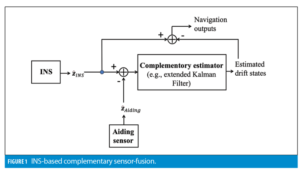
Figure 1 shows a high-level diagram of complementary sensor-fusion with inertial navigation.
The algorithm uses differences between aiding measurements and their INS-based predictions as inputs to the complementary estimator. An Extended Kalman Filter (EKF) is the most common form of the complementary estimation, however, other estimation methods (such as particle filters and factor graphs) have been applied as well.
Example Implementation
To provide insights into complementary filter design aspects, this section considers an example case of loose GNSS/INS integration with the EKF-based fusion. The Kalman filter mechanization is completely defined by (i) state vector X, (ii) state transition matrix F, (iii) process noise covariance Q, (iv) measurement (or observation) vector z, (v) observation matrix H, and (iv) measurement error covariance R. Once these six terms are defined, recursive Kalman filter updates are applied using standard filter equations. The INS error propagation defines the first three terms. The propagation mechanism was considered in a previous Inertialist column (see May/June 2022 issue of Inside GNSS). To complete the integrated system mechanization, we need to define the remaining three terms.
For loose integration, complementary position observables are formulated as differences between INS and GNSS position solutions (rˆINS and rˆGNSS):

where δr is the INS position error and εr is the GNSS position measurement error vectors, respectively. Note the update rate of INS solution is generally higher than that of GNSS. Hence, the observation update at tn is applied only if GNSS position is available at that time. Otherwise, the complementary filter relies on prediction with state estimates being assigned their predicted values.
Additionally, the formulation makes two other simplifications. First, INS and GNSS solutions are assumed to arrive at the exact same time (i.e., stay completely synchronized). Generally, this is not the case and timing adjustments must be made. The adjustment can be performed by propagating INS navigation states to the time of validity of GNSS measurements. Second, the inertial measurement unit (IMU) and GNSS antennas are assumed to be collocated with each other (i.e., their relative lever arm vector is zero). Equation 1 needs to be updated to include a lever-arm term for non-zero lever-arm cases.
The observation matrix H defines how elements of the state vector project into measurement observables. This matrix has a size of K×P, where K is the number of scalar measurements and P is the number of elements in the state vector. For position updates (three position components) and a 15-state INS error model (including position, velocity and attitude errors, and gyro and accelerometer biases), H has a size of 3×15. Position error states directly project into the observation vector, while the contribution of other error states is zero. Hence, the H matrix is formulated as:

where I(3×3) and 0(3×3) are the 3×3 unit matrix and zero matrix, respectively.
Formally, the observation matrix is derived by taking partial derivatives:

where:
Hk,p is the element of the observation matrix that corresponds to its kth row and pth column;
zk is the kth element of the observation vector; and,
Xp is the pth element of the state vector.
It can be readily verified that when partial derivatives of the observation vector in Equation 1 are computed with regard to the elements of the state vector, this results in the observation matrix in Equation 2.
By definition, the measurement error covariance R is:

where E[ ] denotes the mean value and T is the matrix transpose operator.
The Kalman filter assumes that measurement errors are zero-mean Gaussian. R is a diagonal matrix when errors in different GNSS position components are not correlated with each other:
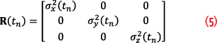
where σx , σy and σz are standard deviations of x, y and z position errors, respectively.
This example of loosely coupled GNSS/INS can be extended to other complementary sensor fusion mechanizations such as tightly coupled GNSS/INS and fusion with other aiding data sources (e.g., bearing angles to visual landmarks at known or unknown locations). The INS system propagation remains the same, but the state vector may have to be augmented by error states associated with the aiding sensor (such as GNSS receiver clock error states and misorientation between the IMU and video camera). The complementary observations are formulated in a similar manner, i.e., as differences between actual aiding measurements and their INS predicted values, for example, between measured and predicted GNSS pseudoranges. The observation matrix H is derived by taking partial derivatives of the measurement observables similarly to Equations 2 and 3. Finally, the measurement noise matrix R is formulated based on measurement noise covariances.
Main Benefits
As compared to the full-state formulation (i.e., direct estimation of the navigation states), the main benefit of a complementary filter for GNSS/INS integration is a significantly simplified modeling of state transition. Inertial errors are propagated over time instead of propagating navigation states themselves. In this case, the process noise covariance matrix, Q, is completely defined by the stability of INS sensor biases, as well as sensor noise characteristics. On the contrary, modeling of actual motion generally needs to accommodate different motion segments (such as a straight flight versus a turn maneuver), which can require ad hoc tuning. An adaptive tuning of the Q matrix may be required to optimize the performance.
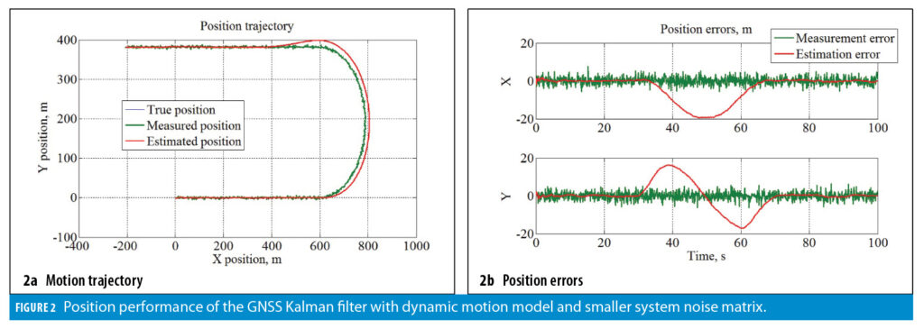
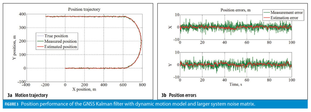
To illustrate this benefit, Figures 2 through 4 show example simulation results. A filtering of noisy GNSS position is considered. The motion trajectory includes two straight segments and a 180 degree turn maneuver. Figures 2 and 3 show outputs of a Kalman filter that does not use the INS and model navigation states instead (more specifically, a constant-velocity motion model is applied). In Figure 2, a smaller value of the system noise matrix (Q-matrix) is used. This allows for an efficient smoothing of GNSS measurement noise. However, during the turn (when non-zero acceleration is introduced and the constant-velocity motion model becomes invalid), position errors increase substantially. Increasing the system noise matrix increases the measurement feedback into the Kalman filter and helps to mitigate the divergence during the turn as shown in Figure 3. However, it comes at a cost of increased estimation noise.
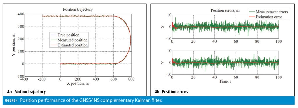
The dynamic modeling/noise smoothing trade-off is eliminated when a complementary GNSS/INS Kalman filter is applied as shown in Figure 4. In this case, the system (i) substantially suppresses the measurement noise (similarly to Figure 2), and (ii) accurately follows the motion dynamic (similarly to Figure 3).
Another benefit of the complementary estimation is the ability to linearize the state propagation and use computationally efficient linear estimation techniques. Specifically, propagation of navigation states through INS mechanization is a non-linear process. In contrast, time-propagation of inertial errors into navigation outputs can be efficiently linearized. As a result, the complementary filter can benefit from linear filtering techniques (such as an extended Kalman filter) without the need for nonlinear estimation methods such as an unscented Kalman filter and particle filter.
Observability of Error States
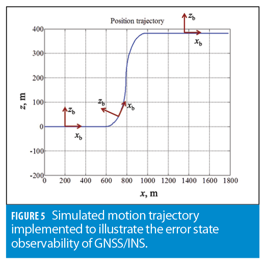
State observability of the complementary sensor-fusion is one of the key aspects influencing system performance. To provide an insight into it, this section considers a two-dimensional (2D) simulation of a loosely coupled GNSS/INS, which is illustrated in Figure 5.
GNSS position updates are used for INS drift mitigation. Acceleration due to gravity is in the direction opposite to the z-axis. The platform has a constant absolute velocity value of 20 m/s. The trajectory starts with a straight motion segment, follows it by a climb (with turning of the IMU body-frame), and completes with a straight motion.
Inertial sensor errors were simulated as follows:
• Gyro drift: first-order Gauss-Markov process, standard deviation is 50 deg/hr, correlation time is 1000 s;
• Accelerometer bias: first-order Gauss-Markov process, standard deviation is 1 mg, correlation time is 1000 s.
GNSS position errors were simulated as zero-mean Gaussian processes with a standard deviation of 1 cm. This position performance corresponds to a carrier phase-based RTK solution. INS and GNSS update rates were 100 Hz and 1 Hz, respectively.
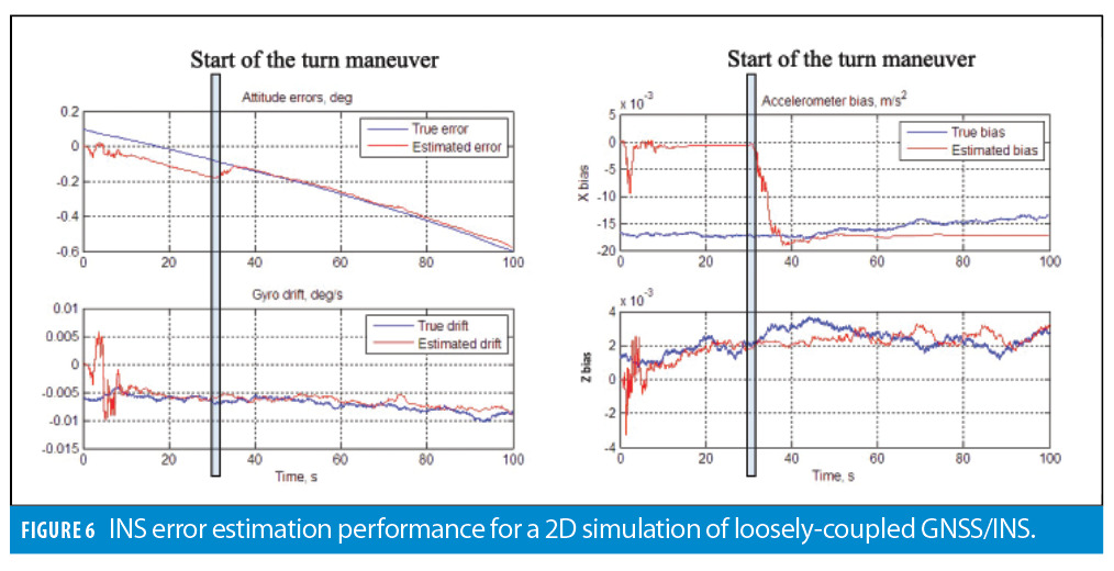
Figure 6 shows estimates of angular errors (attitude and gyro drift) and accelerometer biases.
As shown in Figure 6, attitude error and x-accelerometer bias cannot be estimated separately (residual estimation errors remain) during the initial straight segment. Their estimates converge to true values after the climb starts and sufficient motion dynamics are accumulated for the error state separation.
The plots provide initial insight into the influence of motion dynamics on the observability of INS error states. As shown in Figure 6, there is a residual attitude error that remains uncompensated during the straight motion phase. The estimate of the z-accelerometer bias rapidly converges to its true value while its x-accelerometer counterpart cannot be estimated. Both attitude error and x-accelerometer bias estimates converge to their true values shortly after the climb starts at about 30 seconds into the simulation.
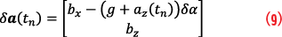
This phenomenon can be explained as follows. Essentially, the Kalman filter numerically differentiates position error states into acceleration error and then separates the latter into attitude and bias error terms. For simplicity, consider a 2D case where (i) body-frame is aligned with the navigation frame; and, (ii) accelerometer biases, b, and angular orientation error, δα, are constant. INS does not take advantage of the known angular orientation (i.e., the fact that body and navigation frames are aligned with each other) and integrates gyro measurements into attitude. In this case, the navigation-frame acceleration error is:

For constant-velocity motion:

The z-bias component can be directly estimated from the z-acceleration error, which, in turn, is estimated from position error observations. However, observations of the x-acceleration error over time are rank-deficient. This does not allow for the separation between bias and attitude error terms. The filter balances their contribution into acceleration error but cannot estimate them individually.
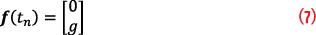
When time-varying acceleration is applied along the z-axis, the observation model in Equation 8 changes into:
When this system is observed over time, it has a full rank and bias and attitude error terms can now be estimated separately. This is what happens in Figure 6 after the platform starts climbing.
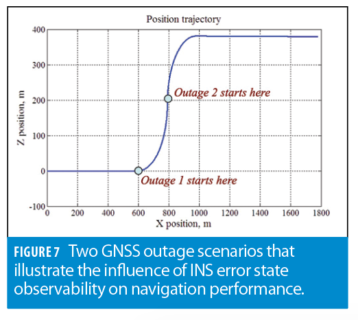
Clearly, when centimeter accurate GNSS position is available all the time, it is not critical to estimate individual INS error terms. However, the observability aspect becomes more critical when GNSS outages are present. To illustrate, we consider two outage scenarios as shown in Figure 7.
Outage 1 starts before the climb when attitude and bias errors cannot be separated. Outage 2 starts during the climb after the sufficient error state convergence is achieved. Figure 8 compares GNSS/INS position performance for these two outage cases.
As shown in Figure 8, INS drift during the second outage is reduced significantly due to the ability to separate attitude and bias error states during the climb maneuver. Particularly, the maximum error growth is reduced (from 2.7 m and 5 m for x and z position components to 0.5 m and 2 cm, respectively) for the second outage scenario. This error reduction is due to the ability to separately estimate angular and linear INS error terms by using the motion dynamics.

Conclusion
Complementary sensor fusion is the most efficient approach to fuse INS with aiding sensors. The methodology (i) models inertial error dynamics rather than modeling full motion states, and (ii) applies differences between actual measurements and their INS-based predictions as estimation observables. One of the key benefits is the ability to use computationally efficient linear estimation techniques (such as an extended Kalman filter) for the error-state propagation. Another benefit is a straight-forward choice of the system noise matrix (that is fully defined by INS error models) without the need to make a trade-off between the system’s ability to suppress the measurement noise and accurately follow a platform’s motion (e.g., during a straight flight and a turn maneuver) dynamics. This column also illustrated that the observability of inertial error states is generally impacted by the motion dynamics, which can have substantial influence on navigation performance during GNSS outages.


