In the past decade, there has been a sharp increase in GNSS outages due to deliberate GNSS jamming. Receivers in LEO are uniquely situated to detect, classify and geolocate terrestrial GNSS jammers. This article explores two-step and direct geolocation of terrestrial GNSS jammers from LEO.
ZACHARY CLEMENTS, TODD E. HUMPHREYS, UNIVERSITY OF TEXAS AT AUSTIN
PATRICK B. ELLIS, APPLE, FORMERLY SPIRE GLOBAL
Global Navigation Satellite Systems (GNSS) such as GPS provide meter-accurate positioning while offering global accessibility and all-weather, radio-silent operation. However, GNSS is fragile: its service is easily denied by jammers or deceived by spoofers [1-3]. GNSS signals are especially vulnerable to jamming because they are extremely weak: near the surface of Earth, they have no more flux density than light received from a 50 W bulb at a distance of 2,000 km [4]. Furthermore, GNSS jammers are easily accessible and low cost, threatening GNSS-reliant systems [5,6]. Without proper countermeasures, victim GNSS receivers can be rendered useless.
The civilian maritime and airline industries frequently encounter GNSS jamming and spoofing. Corrupted Automatic Identification System (AIS) and Automatic Dependent Surveillance-Broadcast (ADS-B) messages from surface vessels and aircraft are often reported. Irregularities in AIS and ADS-B reports are often indicative of GNSS interference. Geolocation of GNSS jammers with ADS-B data is possible, but only coarse jammer position estimates are achievable [7,8].
Recently, the German Aerospace Center (DLR) performed a data collection flight over the Eastern Mediterranean to study the behavior of regular avionics and aviation-grade GNSS receivers under jamming conditions [9]. The DLR also conducted an international maritime measurement campaign to detect GNSS interference [10]. In both studies, the recorded data showed evidence of high-power GNSS jammers, including a chirp jammer centered at the GPS L1 frequency in the Eastern Mediterranean.
A first step to developing situational awareness and eliminating GNSS interference is geolocating the emitters involved. It was shown that a network of ground-based receivers could track and geolocate chirp-style jamming signals in [11] and matched-code jamming signals in [12]. The more general case of localizing an emitter transmitting an arbitrary wideband signal with terrestrial and airborne receivers has been extensively studied [13-16]. However, because the receivers were either at fixed locations or tactically deployed in the nearby airspace, only emitters in the immediate area could be geolocated. There remains a need for global, persistent, low-latency, and accurate GNSS interference detection and localization.
Receivers based in low Earth orbit (LEO) are a proven asset for detecting, classifying and geolocating terrestrial GNSS interference [17-19]. Emitter geolocation from LEO offers worldwide coverage with a frequent refresh rate, making it possible to maintain a common operating picture of terrestrial sources of interference, e.g., GNSS jammers and spoofers. Moreover, LEO satellites’ stand-off distance from terrestrial interference sources typically permits tracking authentic GNSS signals, enabling precise time-tagged data captures from time-synchronized LEO-based receivers and precise orbit determination. LEO constellations with distributed time-synchronized receivers can provide unprecedented emitter geolocation. Several commercial enterprises have seized the opportunity to provide spectrum monitoring and emitter geolocation as a service (e.g., Spire Global and Hawkeye360).
Accurate single-satellite-based emitter geolocation is possible from Doppler measurements alone, provided the emitter’s carrier can be extracted [18-20]. Performance bounds and error
characterization for Doppler-based single-satellite geolocation are presented in [21, 22]. However, accurately locating emitters with arbitrary waveforms using a single LEO receiver is impossible in general: If the signal’s carrier cannot be tracked, only coarse received-signal-strength techniques can be applied for geolocation.
On the other hand, geolocation of emitters producing arbitrary wideband signals is possible and has been extensively studied [13, 23, 24]. Multiple time-synchronized receivers can exploit time- and frequency-difference of arrival (T/FDOA) measurements to estimate the emitter location. Geolocation based on T/FDOA is typically a two-step process. First, a time series of T/FDOA measurements is produced by correlating captured signals against another. Second, the time series is fed to a nonlinear estimation algorithm to geolocate the source. Two-step T/FDOA has been previously applied for terrestrial emitter localization from geostationary orbit [25].
One weakness of two-step geolocation is it ignores the constraint that all measurements must be consistent with a single position in the case of a stationary emitter, or a single trajectory in the case of a moving emitter [26]. A second weakness of the two-step approach is interference signals exhibiting
cyclostationarity give rise to structures in the T/FDOA measurement domain that make it harder to track individual emitters. Identification and tracking becomes especially challenging when there are multiple cyclostationary emitters with overlapping frequency content and a wide range of received power, in which case the T/FDOA measurement domain becomes highly structured with features ambiguously related to the emitters involved.
Another multi-receiver technique is direct geolocation, which is a single-step search over a geographical grid to estimate a transmitter’s location directly from the observed signals [26-30]. In direct geolocation, the TDOA and FDOA are directly parameterized for a single geographical point, given knowledge of the receivers’ position, velocity and clock states. Direct geolocation outperforms the two-step method in low signal-to-noise ratio (SNR) environments and in short-data-capture scenarios, making it ideal for LEO-based geolocation. Furthermore, as will be shown in this article, direct geolocation is better suited for processing captures with cyclostationary signals from multiple emitters, because rather than searching in the T/FDOA measurement domain cluttered by overlapping structures, it searches in the position domain, where individual emitters are separated by their physical distance, irrespective of any time correlation in their signals.
This article demonstrates two-step and direct geolocation on raw intermediate frequency (IF) samples recorded from Spire Global’s LEO constellation. For the first time in the open literature, real-world GNSS narrowband, matched-code, and chirp jamming signals captured by two time-synchronized LEO receivers are characterized and their emitters geolocated.
Measurement Model
TDOA and FDOA Measurement Model
Let pi(t) and vi(t) denote the position and velocity vector for the ith receiver, and pe denote the emitter’s position vector, all in a common rectangular coordinate frame. In this model, the emitter is assumed to be stationary. The time of arrival (TOA) at the ith receiver of the signal transmitted from the emitter at time t is modeled as
where the range vector ri(t) between the emitter and the ith receiver is

The range between the emitter and the ith receiver is related to τi and ri by

Finally, the unit vector from emitter position to the ith receiver position is defined as

Different LEO-based receivers will receive the same signal at different times due to the differing geometry between receivers. Assuming the receivers are synchronized to GPS time, the time difference of arrival (TDOA) of the same signal between the ith and jth receiver is defined as

which can be converted to a range difference by multiplying by the speed of light.
The frequency of arrival (FOA) measurement is synonymous with the received Doppler of a signal. For a stationary emitter, the FOA on the ith moving receiver is composed of three components: (1) the range-rate between the emitter and receiver (2) the clock offset rate of the receiver
, and (3) the clock offset rate of the emitter
. The FOA at the ith receiver is modeled as

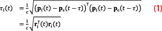
Different LEO receivers will also receive the same signal at different frequencies due to the differing instantaneous range-rates and receiver clock offset rates. Let denote the frequency difference of arrival that includes the receivers’ clock offset rates.
An advantageous feature of is the clock offset rate from the emitter is removed: because the same emitter clock offset rate is observed at each receiver, it gets canceled out in the differencing. The approximation disregards the
and
cross terms, as they are negligible. The frequency difference of arrival (FDOA) Δf(t) with compensated receiver clock offset rate between the first and second receiver is defined as
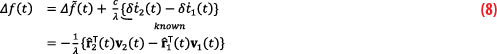
The FDOA measurement is the difference between range-rates scaled by the negative reciprocal of wavelength.
The Generalized Cross-Correlation Function
Assume all receivers are synchronized to GPS time and clock errors have been compensated for. The generalized cross-correlation function (GCCF) for a pair of received complex baseband signals y1(t) and y2(t) is

where T is the integration interval. The more familiar complex ambiguity function (CAF) from the radar literature [31] with constant delay τ0 and Doppler fd is

This can be expressed in terms of the GCCF by τ1(t)=0 and τ2(t)=. Over short intervals, the errors introduced by assuming the delay τ0 and Doppler fd to be constant are negligible [28]. The maximum coherent integration length T is typically dictated by the receivers’ dynamics and clock variations.
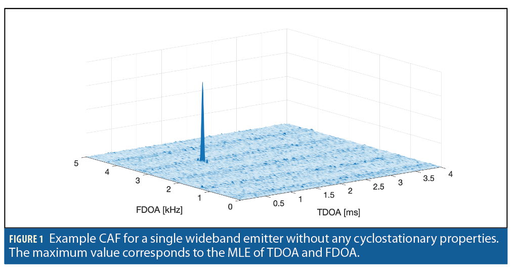
Consider a pair of spatially separated receivers with received signals y1(t) and y2(t). If there is only a single emitter, it is shown in [27,32] that the delay and Doppler that maximizes the magnitude of the CAF, denoted as τ0=Δt and fd =Δf, are the corresponding maximum likelihood estimates (MLE) of the time and frequency difference of arrival between a pair of receivers. Figure 1 is an example CAF.
Several complications arise when there are multiple emitters present. In this case, the auto-ambiguity terms generated by each emitter’s waveform may interfere with each other, leading to biases in the T/FDOA estimate [27]. Moreover, the height of an emitter’s peak in the CAF is determined by the emitter’s transmit power. Weaker emitters will have smaller peaks, leading to possible missed detections in the presence of stronger emitters. Furthermore, transmitted signals exhibiting cyclostationarity give rise to additional structures in the CAF, making individual peaks more difficult to track.
Emitter Geolocation with Two-Step and One-Step Techniques
Two-Step Geolocation
In the traditional two-step geolocation approach, a time series of T/FDOA measurements is first obtained by repeated CAF generation and peak tracking. The CAF is computed at each time instant a T/FDOA measurement is desired. For model simplicity, TDOAs can be converted to range difference in meters by scaling them by the speed of light. FDOAs can be converted to range-rate in meters per second by scaling by −λ.
All dual-satellite emitter geolocation techniques assume the emitter altitude is constrained to strengthen observability. This article takes a straightforward approach: the receivers’ positions and velocity are converted into the East-North-Up (ENU) frame centered at the current best estimate of the emitter’s position, i.e., pe=[0,0,0]T. The emitter’s position is now in a state that is easily related to the measurement model and the altitude is constrained because the up coordinate is held to 0.
A nonlinear least-squares (NLLS) estimator is used to solve for the position of the transmitter. The standard weighted nonlinear least-squares cost function is

where x is the 2×1 state representing the emitter’s position, and x and y respectively denote the displacement east and north from the current best estimate

z is the 2N×1 T/FDOA measurement vector
h(x) is the 2N×1 nonlinear measurement model function
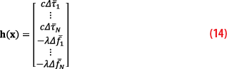
where Δτ–k and Δf–k are the estimates of Δτk and Δfk at the current best estimate of the state, and k denotes the kth T/FDOA measurement pair. R is the 2N×2N measurement covariance matrix with the variance of the TDOA measurements along the first N diagonal elements and the variance of the FDOA measurements
along the second N diagonal elements.
One of the most common ways to solve the standard nonlinear least-squares problem is with the Gauss-Newton method. Because this estimator is operating in the ENU frame, two additional steps must be taken. A possible implementation of two-step geolocation starting from raw samples to final emitter position estimate is presented in the full paper. This two-step T/FDOA geolocation model also can be reduced to a TDOA-only solution or a FDOA-only solution. Those solutions can be used as a reasonableness test for the combined T/FDOA solution and to quantify the accuracy of the TDOA and FDOA measurements.
Direct Geolocation
The direct geolocation approach is a single-step grid-search method that solves directly for the emitter position without the need for intermediate T/FDOA measurements. The CAF is maximized directly by parameterizing the delay and Doppler time histories in terms of the emitter’s position, as well as the known receivers’ position, velocity and clock time histories. The direct approach outperforms the two-step approach in low SNR regimes and in cases limited to short captures.
A grid of three-dimensional emitter positions must be first designated. One approach is to create a grid in latitude and longitude. Then, for each latitude and longitude pair, the altitude can be retrieved from a terrain model. This constrains the emitter position to the relative terrain on the surface of the Earth. Given that the emitter’s position is assumed, and that the time history of the receivers’ position, velocity and clock offset rate are known, the time history of TOAs and FOAs of a transmitted signal at each receiver can be computed with (1) and (6). It follows that a time history of TDOA and FDOA can be computed using (5) and (8).
Consider a time-synchronized capture between two receivers lasting T seconds producing Ns samples. Let fs represent the sampling rate and Ts the time between samples. The digital representation of the signal yi(t) is given by yi[k]=yi(kTs). A time history of TDOA Δτ and FDOA Δf measurements can be computed at each sample for every emitter position. The TDOA and FDOA are not constant over long integration intervals, thus, a comprehensive model for the non-constant TDOA and FDOA time history is required.
Recall that a signal’s instantaneous frequency is the time derivative of the phase f(t)=dθ(t)/dt. Let ΔΘ denote the Ns×1 vector containing a phase shift for each sample. For intervals with a time-varying FDOA, a polynomial approximation of the FDOA time history is computed. A polynomial approximation to Δf is taken, and then integrated to get a phase shift time history ΔΘ.
Let denote the integer sample offset vector corresponding to Δτ, where
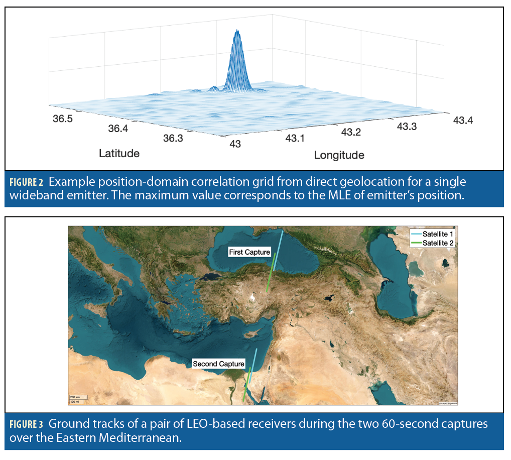
denotes the round function. Let Δτ~k and ΔΘk denote the kth element of Δτ∼ and ΔΘ, respectively. The position-domain correlation value at a grid point is defined as
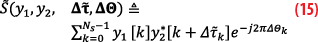
The position corresponding to the Δτ∼ and Δf values that maximize |S~(y1,y2,Δτ∼,ΔΘ)| is the maximum-likelihood emitter location. Figure 2 shows an example of direct geolocation. An example implementation is presented in the full paper.
One of the main advantages of the direct approach is it enables longer coherent integration intervals of the received signals compared to the basic CAF in the two-step approach. For longer coherent integration times, the peak at the true emitter position becomes sharper and more pronounced. Another advantage of direct positioning is there will be a peak at every position where an emitter is located, provided the emitter’s signal was strong enough to be received at both receivers. Finally, this technique works for any waveform—including those exhibiting cyclostationarity. Noncoherently combining position-domain correlations prunes any structures due to repetition in the transmitted waveform as well as any spurious peaks due to noise.
A Recent Real-World Capture
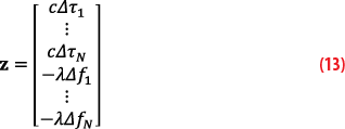
This section describes the dual-receiver platform and spectral characteristics of two capture events over the Eastern Mediterranean in April 2022.
Spire Satellites
Spire has a vast network of LEO satellites helping ensure global coverage and near-real-time data collection. Their satellites and geolocation solutions offer superior visibility and accuracy for monitoring maritime activities and tracking signals of interest. Among these satellites are about 60 STRATOS satellites, whose original purpose was GNSS radio occultation (GNSS-RO), that can be repurposed for geolocation of emitters operating in the GPS L1 and L2 bands. The STRATOS satellites carry one wide-field-of-view zenith-facing antenna for precise orbit determination, and one or two Earth-limb-facing narrow-field-of-view high-gain antennas. STRATOS’s RF circuitry has three dual-frequency channels, with each antenna connected to one of the front end channels. Digitization of each signal happens coherently based on a single sampling clock. Simultaneous collections of the 2-bit quantized 6.2 Msps raw intermediate frequency (IF) samples centered at GPS L1 and L2 can be performed. These data can be packaged and downlinked through Spire’s network of dedicated ground stations.
In April 2022, two STRATOS satellites performed two consecutive 60-second simultaneous capture events separated by 180 seconds while over the Eastern Mediterranean as shown in Figure 3. During each 60-second capture, the satellites had an average altitude of 524 km and an average velocity of 7,678 m/s, traveling from north to south. The raw samples from the GNSS-RO antennas and the onboard navigation solution were downlinked for post-processing.
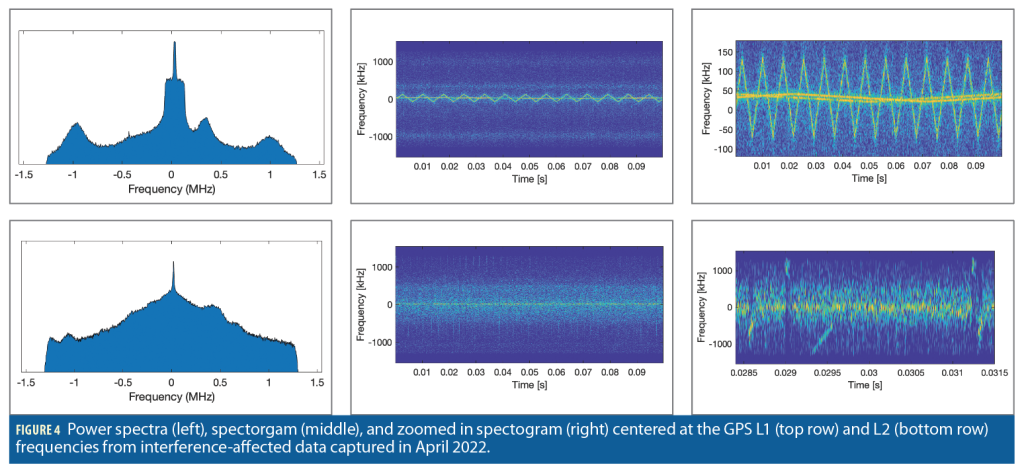
Spectrum Analysis
Figure 4 illustrates the captured signals’ spectral characteristics during the first simultaneous capture event. There is composite wideband interference on both GPS L1 and L2. Visual inspection of the spectogram indicate that L1 contains multiple CW chirp jammers as well as other wideband interference. The wider-bandwidth chirp jammer had a bandwidth of approximately 200 kHz and a period of 7.7 ms. The narrower-bandwidth chirp jammers had a bandwidth of approximately 20 kHz and a period of 100 ms. The 20 kHz chirp jammers have the same parameters of a jammer previously captured in the Eastern Mediterranean [10]. L2 contains a particularly strong narrowband jammer as well as other wideband interference. Throughout the captures, multiple long range air surveillance radars operating near GPS L2 are visible.
Emitter Geolocation
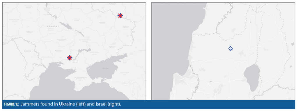
This section discusses two-step and direct geolocation of the emitters captured in the Spire dataset. The results focus on the geolocation of a known GNSS jammer operating out of Khmeimim Air Base on the coast of Syria. Wide-area GNSS interference monitoring via direct geolocation reveals numerous jammers across Syria, Turkey, Iraq, Ukraine and Israel.
Two-Step Geolocation
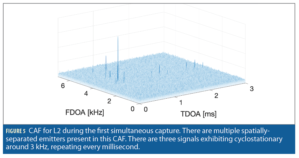
In the L2 CAF, there are multiple spatially-separated emitters present. The more spatially diverse the emitters are, the more separated the peaks in the CAF become. Additionally, cyclostationary signals manifest repeating patterns in the CAF, as shown by the run of peaks around 3 KHz in Figure 5.
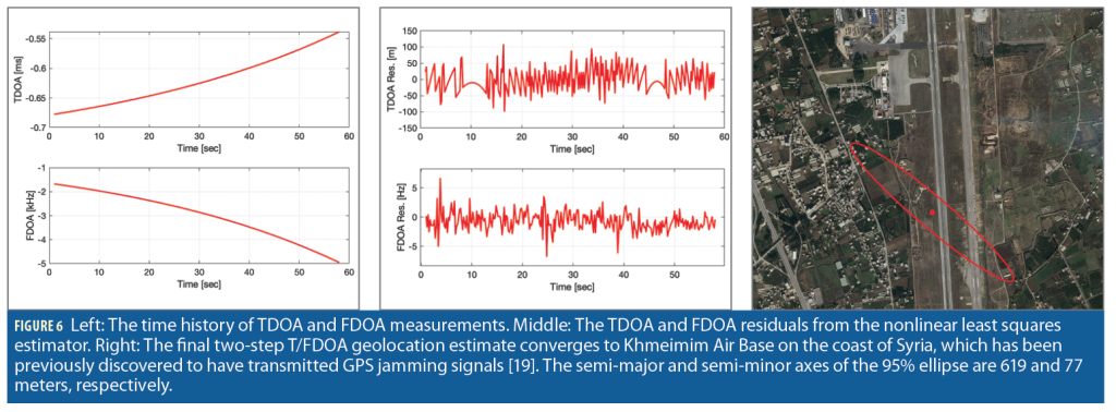
Figure 6 shows the time history of TDOA and FDOA measurements corresponding to the largest peak in the L2 CAF over the 60- second capture. These measurements were taken at 5 Hz and then served to the nonlinear estimator. The final two-step emitter position estimate is displayed in Figure 6. The final solution converged to Khmeimim Air Base on the coast of Syria, which has been previously discovered to host a powerful GPS jammer [18].
The TDOA and FDOA residuals from the nonlinear least-squares estimator are also shown in Figure 6. They are zero-mean and Gaussian distributed, indicating the presented measurement model is accurate. The TDOA residuals time history appears to have unexpected structure; this structure arises due to the range resolution from the sampling rate. Because the sampling rate at baseband is 3.1 Msps, the range resolution is 96.7 m. As a consequence, the TDOA residuals appear to have structure. The TDOA residuals remain between the range resolution of ± 96.7 m, meaning the expected performance with the sampling rate was achieved.
Effects of Signal Cyclostationarity
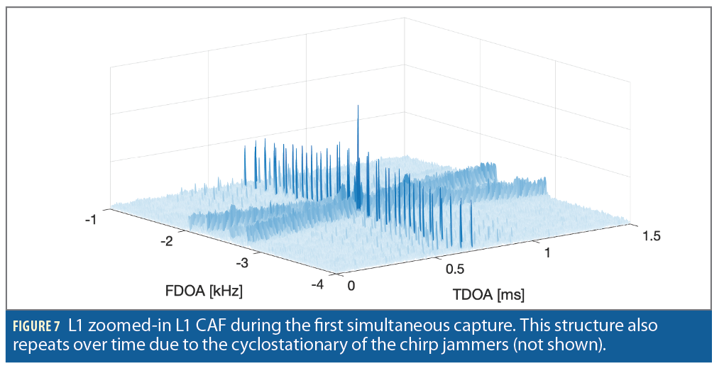
Cyclostationary signals, such as chirp jammers, give rise to structures in the CAF that make it harder to track individual emitters. Identification and tracking becomes especially challenging when there are multiple cyclostationary emitters with overlapping frequency content and a wide range of received power, in which case the T/FDOA measurement domain becomes highly structured with features ambiguously related to the emitters involved. The L1 CAF is shown in Figure 7. Recall that the strongest signals on L1 are the chirp jammers.
Direct Geolocation
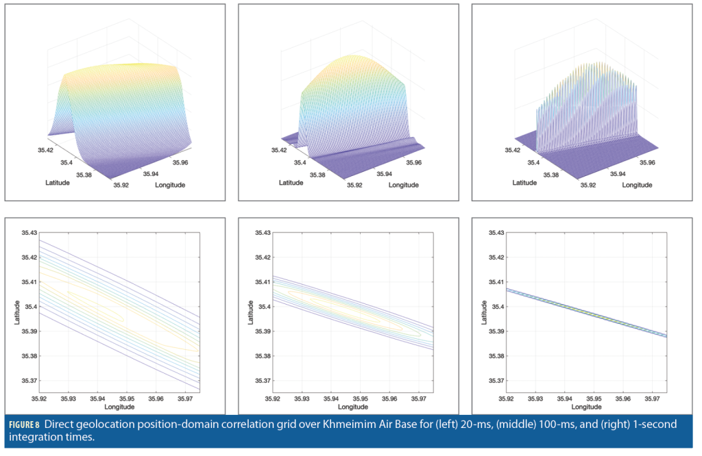
Figure 8 shows the position-domain correlation values over the Khmeimim Air Base using the L2 raw samples with various integration times. For each latitude and longitude pair, the surface altitude was retrieved from a terrain model. The global elevation model used was the Global Multi-resolution Terrain Elevation Data 2010 (GMTED2010) developed by the U.S. Geological Survey and the National Geospatial-Intelligence Agency.
The maximum peak in the position-domain correlation function for the various integration intervals in Figure 8 is nearly equivalent to the two-step solution. In the one-step approach, the effects of integration interval length are apparent in Figure 8. As the integration time increases, the peak becomes sharper and more pronounced. The overall shape of the peak changes with the receiver geometry.
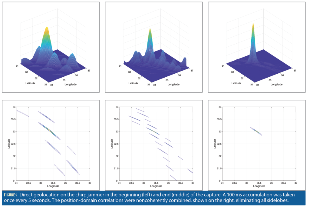
Figure 9 demonstrates how direct geolocation is better suited for processing captures with structured, cyclostationary signals. The position-domain correlation function for the chirp jammer is shown at the beginning (top graph) and end (middle graph). There is structure in both, but that structure changes with the instantaneous receivers’ geometry, which changes over time. When multiple position-domain accumulations are noncoherently combined, all of the false peaks are reduced below the noise floor, while the main peak corresponding to the true emitter position remains. Noncoherent integration is a powerful tool that can suppress spurious false peaks from waveform structure and cyclostationarity.
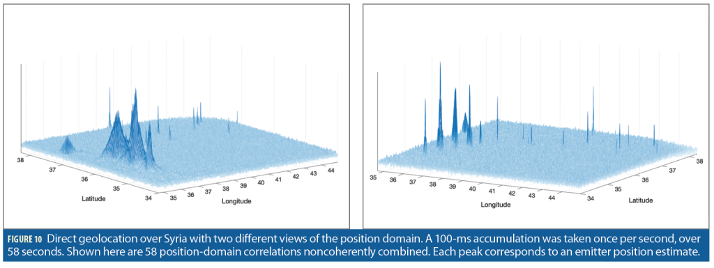
Figure 10 shows direct geolocation over Syria with the L2 data. A 100 ms accumulation was taken once per second, over 58 seconds. The 58 position-domain correlations were noncoherently combined. Each peak corresponds to an emitter position estimate, with the largest peak corresponding to Khmeimim Air Base. The receivers’ geometry also heavily affects correlation in the position domain. There was better receiver geometry for the transmitters on the east-side, resulting in sharper peaks.
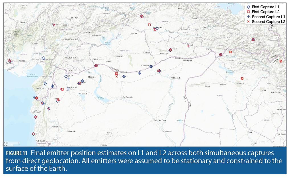
This position-domain correlation was repeated for L1 on the first capture and L1 and L2 on the second capture. The peaks from the position domain correlations on both captures and frequencies are shown in Figure 11. Each one of these estimates is plausible, given the agreement between both frequencies and passes, as well as the surrounding equipment near each estimate. This also showcases the superiority of the direct approach in crowded signal environments. The two-step approach would have depended on an additional complex multi-peak tracking and association algorithm to generate a time series of T/FDOA measurements, whereas in the direct approach the emitter position estimate comes directly from the raw samples.
Conclusion
This article explored two-step and direct geolocation of terrestrial emitters from LEO. It was demonstrated that the direct approach is a powerful geolocation technique for low SNR signals with multiple emitters. We also investigated emitter geolocation in crowded signal environments and explored geolocating cyclostationary signals. Finally, this article demonstrated two-step and direct geolocation on raw intermediate frequency samples. Recent real-world GNSS interference signals captured by two time-synchronized LEO receivers over the Eastern Mediterranean were characterized and their emitters geolocated. The full paper can be found in [33].
Acknowledgments
Research was sponsored by the U.S. Department of Transportation (USDOT) under the University Transportation Center (UTC) Program Grant 69A3552047138 (CARMEN), and by affiliates of the 6G@UT center within the Wireless Networking and Communications Group at The University of Texas at Austin.
References
(1) T. E. Humphreys, “Statement on the vulnerability of civil unmanned aerial vehicles and other systems to civil GPS spoofing,” United States House of Representatives Committee on Homeland Security: Subcommittee on Oversight, Investigations, and Management, July 2012.
(2) M. L. Psiaki and T. E. Humphreys, “GNSS spoofing and detection,” Proceedings of the IEEE, vol. 104, no. 6, pp. 1258–1270, 2016.
(3) Z. Clements, J. E. Yoder, and T. E. Humphreys, “Carrier-phase and IMU based GNSS spoofing detection for ground vehicles,” in Proceedings of the ION International Technical Meeting, Long Beach, CA, 2022, pp. 83–95.
(4) T. E. Humphreys, “Interference,” in Springer Handbook of Global Navigation Satellite Systems. Springer International Publishing, 2017, pp. 469–503.
(5) D. Borio, C. O’Driscoll, and J. Fortuny, “GNSS jammers: Effects and countermeasures,” in 2012 6th ESA Workshop on Satellite Navigation Technologies (Navitec 2012) & European Workshop on GNSS Signals and Signal Processing. IEEE, 2012, pp. 1–7.
(6) Z. Clements, J. E. Yoder, and T. E. Humphreys, “GNSS Spoofing Detection: An Approach for Ground Vehicles Using Carrier-Phase and Inertial Measurement Data,” GPS World, vol. 34, no. 2, pp. 36–41, 2023.
(7) Z. Liu, S. Lo, T. Walter, and J. Blanch, “Real-time detection and localization of GNSS interference source,” in Proceedings of the 35th International Technical Meeting of the Satellite Division of The Institute of Navigation (ION GNSS+ 2022), 2022, pp. 3731–3742.
(8) M. Dacus, Z. Liu, S. Lo, and T. Walter, “Improved RFI localization through aircraft position estimation during losses in ADS-B reception,” in Proceedings of the 35th International Technical Meeting of the Satellite Division of The Institute of Navigation (ION GNSS+ 2022), 2022, pp. 947–957.
(9) O. Osechas, F. Fohlmeister, T. Dautermann, and M. Felux, “Impact of GNSS-band radio interference on operational avionics,” NAVIGATION: Journal of the Institute of Navigation, vol. 69, no. 2, 2022.
(10) E. P. Marcos, A. Konovaltsev, S. Caizzone, M. Cuntz, K. Yinusa, W. Elmarissi, and M. Meurer, “Interference and spoofing detection for GNSS maritime applications using direction of arrival and conformal antenna array,” in Proceedings of the 31st International Technical Meeting of The Satellite Division of the Institute of Navigation (ION GNSS+ 2018), 2018, pp. 2907–2922.
(11) R. Mitch, M. Psiaki, and T. Ertan, “Chirp-style GNSS jamming signal tracking and geolocation,” NAVIGATION: Journal of the Institute of Navigation, vol. 63, no. 1, pp. 15–37, 2016.
(12) J. A. Bhatti, T. E. Humphreys, and B. M. Ledvina, “Development and demonstration of a TDOA-based GNSS interference signal localization system,” in Proceedings of the IEEE/ION PLANS Meeting, April 2012, pp. 1209–1220.
(13) D. Musicki, R. Kaune, and W. Koch, “Mobile emitter geolocation and tracking using TDOA and FDOA measurements,” Signal Processing, IEEE Transactions on, vol. 58, no. 3, pp. 1863–1874, March 2010.
(14) H. Witzgall, “Two-sensor tracking of maneuvering transmitters,” in 2018 IEEE Aerospace Conference. IEEE, 2018, pp. 1–7.
(15) N. Okello, “Emitter geolocation with multiple UAVs,” in 2006 9th International Conference on Information Fusion. IEEE, 2006, pp. 1–8.
(16) R. J. Bamberger, J. G. Moore, R. P. Goonasekeram, and D. H. Scheidt, “Autonomous geolocation of RF emitters using small, unmanned platforms,” Johns Hopkins APL technical digest, vol. 32, no. 3, pp. 636–646, 2013.
(17) D. M. LaChapelle, L. Narula, and T. E. Humphreys, “Orbital war driving: Assessing transient GPS interference from LEO,” in Proceedings of the ION GNSS+ Meeting, St. Louis, MO, 2021.
(18) M. J. Murrian, L. Narula, P. A. Iannucci, S. Budzien, B. W. O’Hanlon, S. P. Powell, and T. E. Humphreys, “First results from three years of GNSS interference monitoring from low Earth orbit,” Navigation, Journal of the Institute of Navigation, vol. 68, no. 4, pp. 673–685, 2021.
(19) Z. Clements, P. Ellis, M. L. Psiaki, and T. E. Humphreys, “Geolocation of terrestrial GNSS spoofing signals from low Earth orbit,” in Proceedings of the ION GNSS+ Meeting, Denver, CO, 2022, pp. 3418–3431.
(20) P. Ellis, D. V. Rheeden, and F. Dowla, “Use of Doppler and Doppler rate for RF geolocation using a single LEO satellite,” IEEE Access, vol. 8, pp. 12 907–12 920, 2020.
(21) P. B. Ellis and F. Dowla, “Single satellite emitter geolocation in the presence of oscillator and ephemeris errors,” in 2020 IEEE Aerospace Conference. IEEE, 2020, pp. 1–7.
(22) P. Ellis and F. Dowla, “Performance bounds of a single LEO satellite providing geolocation of an RF emitter,” in 2018 9th Advanced Satellite Multimedia Systems Conference and the 15th Signal Processing for Space Communications Workshop (ASMS/SPSC). IEEE, 2018, pp. 1–5.
(23) A. Sidi and A. Weiss, “Delay and Doppler induced direct tracking by particle filter,” Aerospace and Electronic Systems, IEEE Transactions on, vol. 50, no. 1, pp. 559–572, January 2014.
(24) K. Ho and Y. Chan, “Geolocation of a known altitude object from TDOA and FDOA measurements,” IEEE Transactions on Aerospace and Electronic Systems, vol. 33, no. 3, pp. 770–783, July 1997.
(25) D. Haworth, N. Smith, R. Bardelli, and T. Clement, “Interference localization for EUTELSAT satellites–the first European transmitter location system,” International journal of satellite communications, vol. 15, no. 4, pp. 155–183, 1997.
(26) A. Weiss, “Direct geolocation of wideband emitters based on delay and Doppler,” Signal Processing, IEEE Transactions on, vol. 59, no. 6, pp. 2513–2521, June 2011.
(27) J. Bhatti, “Sensor deception detection and radio-frequency emitter localization,” Ph.D. dissertation, The University of Texas at Austin, Aug. 2015.
(28) A. M. Reuven and A. J. Weiss, “Direct position determination of cyclostationary signals,” Signal Processing, vol. 89, no. 12, pp. 2448–2464, 2009.
(29) J. Li, L. Yang, F. Guo, and W. Jiang, “Coherent summation of multiple short-time signals for direct positioning of a wideband source based on delay and Doppler,” Digital Signal Processing, vol. 48, pp. 58–70, 2016.
(30) T. Tirer and A. J. Weiss, “High resolution localization of narrowband radio emitters based on Doppler frequency shifts,” Signal Processing, vol. 141,
pp. 288–298, 2017.
(31) A. Rihaczek, Principles of high-resolution radar. McGraw-Hill, 1969.
(32) S. Stein, “Differential delay/Doppler ML estimation with unknown signals,” Signal Processing, IEEE Transactions on, vol. 41, no. 8, pp. 2717–2719, Aug. 1993.
(33) Z. Clements, P. Ellis, and T. E. Humphreys, “Dual-satellite geolocation of terrestrial GNSS jammers from low Earth orbit,” in Proceedings of the
IEEE/ION PLANS Meeting, Monterey, CA, 2023, pp. 458–469.
Authors
Zachary Clements (B.S., Clemson University; M.S., University of Texas at Austin) is a graduate student in the department of Aerospace Engineering and Engineering Mechanics at The University of Texas at Austin, and a member of the UT Radionavigation Laboratory. His research interests include GNSS signal processing, software-defined radio, and statistical estimation with an emphasis on secure, robust and precise perception. He won the 2023 IEEE Walter Fried Award for best paper at the IEEE/ION PLANS conference for his work on RF interference detection, classification and geolocation from low Earth orbit.
Todd E. Humphreys (B.S., M.S., Utah State University; Ph.D., Cornell University) holds the Ashley H. Priddy Centennial Professorship in Engineering in the department of Aerospace Engineering and Engineering Mechanics at the University of Texas at Austin. He is Director of the Wireless Networking and Communications Group and of the UT Radionavigation Laboratory, where he specializes in the application of optimal detection and estimation techniques to positioning, navigation and timing. His awards include the UT Regents’ Outstanding Teaching Award (2012), the NSF CAREER Award (2015), the ION Thurlow Award (2015), and the PECASE (NSF, 2019). He is Fellow of the ION and of the RIN.
Patrick B. Ellis (M.S., Ph.D., Univ. of California at Santa Cruz; B.S. Bradley University) is currently a GNSS Wireless Systems Engineer at Apple. There he specializes in statistical signal processing, algorithmic development, physics-based modeling, and sensor fusion. Previously, he was the Technical Lead of the Signal Processing Group at Spire Global, where he designed and led solutions for LEO space-based geolocation across many RF bands spanning many government and private programs. Additionally, he was a Senior Research Engineer at the Southwest Research Institute where he worked in the Defense & Intelligence Solutions Division on ionospheric array signal processing projects.


