Dual-frequency PPP GNSS and MEMS-IMU Integration For Continuous Navigation in Obstructed Environments

This article investigates and analyzes position solution availability and continuity from integrating low-cost, dual-frequency GNSS receivers using PPP processing with the latest low-cost, MEMS IMUs. The integration offers a complete, low-cost navigation solution that will enable during GNSS signal outages of half a minute, with a 30% improvement over low-cost, single-frequency GNSS-PPP with MEMS IMU integrations previously demonstrated. This can apply to UAVs, pedestrian navigation, autonomous vehicles, and more.

By Sudha Vana, Nacer Naciri and Sunil Bisnath, York University, Toronto

Integration of inertial measurement units (IMUs) with GNSS helps to achieve continuous navigation in sky-obstructed environments with increased frequency of solution availability. Advancements in micro-electro-mechanical sensors (MEMS) technology has led to the development of low-cost, good performance IMUs. MEMS-based IMUs are inexpensive but have limited stability due to higher noise levels, biases, and drifts.

In the past, most researchers using MEMS-based IMUs used differential GPS (DGPS) and real-time kinematic (RTK) techniques to attain higher accuracy, or high-performance GNSS receivers with the precise point positioning (PPP) technique. PPP technology, as a wide-area augmentation approach, does not require any local ground infrastructure such as continuous operating reference stations. Accuracy attained is at the decimeter to centimeter level in static mode, which approaches RTK performance.

This approach is widely accepted as reliable for precise positioning applications such as crustal deformation monitoring, precision agriculture, airborne mapping, marine mapping and construction applications, and high-accuracy kinematic positioning.

Although the GNSS PPP-only position solution has the drawback of slow initial convergence time, its accuracy makes it attractive for use in applications such as autonomous vehicles, drones, augmented reality, pedestrian navigation, UAVs and other emerging scientific, engineering and consumer applications. These applications demand continuous position accuracy in the order of the meter to centimeter range to satisfy safety, integrity and security requirements.

For instance, in autonomous vehicle navigation systems, lane-level navigation requires very stringent accuracy in the order of centimeters. Here we develop precise, continuous and accurate position solutions using low-cost, dual-frequency GNSS PPP and low-cost MEMS IMU for contemporary applications. We analyze this technique’s performance in realistic obstructed environments.

Using a dual-frequency GNSS receiver—as opposing to single-frequency GNSS investigated in previous research—mitigates the ionosphere refraction error. Accuracy improves to the decimeter level by using GNSS observable linear combinations and the PPP processing technique. A low-cost, dual-frequency PPP solution integrated with a MEMS IMU forms an ideal combination for a total low-cost, high-accuracy solution that will potentially open a new window for modern day applications.

In this tightly coupled integration, raw measurements from sensors are used to integrate, producing a more complex algorithm than loosely coupled integration.

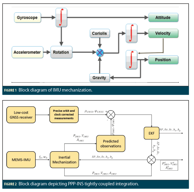
Inertial Mechanization

IMU mechanization is the technique of converting the raw IMU measurements into position, velocity and attitude information. Four steps convert the specific force and turn rates from accelerometers and gyroscopes to position, velocity and attitude. The mechanization also needs initial position, velocity and attitude as references. The four steps in brief are:

• Attitude update;

• Converting specific force from body frame to respective frame in which the mechanization is being performed;

• Velocity update which includes converting specific force into acceleration using a gravity model; and

• Position update.

These four steps of the IMU mechanization are depicted in Figure 1.

This research uses an Earth-centered, Earth-fixed (ECEF) coordinate frame. This is simpler in terms of not having to use conversion while performing the integration, since GNSS measurements are received in terms of distance. The conversion to the necessary coordinate frames can be performed after the integration solution is attained. Inputs to these equations are fb(specific force) and ωibb (turn rates). Below are the ECEF equations for the mechanization process. re is the position, ve is the velocity and Rbe is the attitude of an IMU.

Where, ωibb = Rbeωibe and local gravity vector is ge=Ge(r)- . Initial conditions for initial position (re(0)), velocity (ve(0)) and attitude (Rbe(0)) need to be supplied.

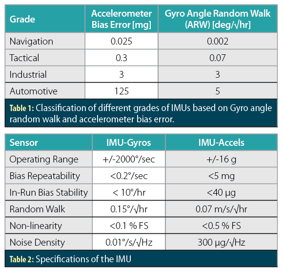
GNSS-PPP/INS Integrated Filter

A tightly coupled architecture here uses an extended Kalman filter to integrate YorkU GNSS-PPP with a MEMS IMU. YorkU GNSS-PPP is a triple-frequency and multi-constellation capable positioning software. In a tightly-coupled architecture, raw measurements from sensors are taken as input to generate corrected states to one of the sensors.

Figure 2 shows the tightly coupled architecture. The inputs to the Extended Kalman Filter are

• the pseudorange and carrier-phase measurements from the low-cost GNSS receiver corrected with the precise orbit and clocks to correct the satellite and orbit errors, and

• predicted pseudorange and carrier-phase measurements formed using the MEMS-IMU position and satellite positions. A part of the state vector consists of the error in position, velocity and attitude that is fed back to inertial mechanization block to close the loop.

fb, wb are the specific force and turn rate measurements from the inertial measurement unit which constitute inputs to the mechanization block. With initial position and velocity from GNSS as input to the mechanization block, PIMU,VIMU and AIMU are position, velocity and attitude from the IMU. Using satellite positions which are corrected using the precise orbit and clock corrections, predicted pseudorange and carrier-phase measurements (ρIMU,φIMU) are formed. ρGNSS, φGNSS are GNSS pseudorange and carrier-phase measurements corrected for orbit and clock errors using precise orbit and clock products. The dual-frequency (L1 and L2) GNSS measurements are used in the ionosphere-free combination to remove the ionosphere refraction error. The difference or residuals between the GNSS measurements and the predicted measurements are processed in the EKF to produce error in position, velocity and attitude states of the sensor which is represented as δP, δv, δε, bg and ba. The IMU error states are used in the mechanization block to continuously correct the errors. The final integrated position, velocity and attitude from an IMU are represented by and .

System Model

The system model in continuous form can be represented as:

δx is the state vector with a combination of navigation, inertial and GNSS states:

• Navigation states: three position error states, three velocity error states and three attitude error states.

• Inertial states: accelerometer and gyroscope biases, accelerometer and gyroscope scale factors.

• GNSS states: troposphere wet delay, GNSS receiver clock, as well as drift and the ambiguity terms.

The states are detailed in mathematical terms as:

where

δP–3D position error vector in the ECEF frame

δv–3D velocity error vector in the ECEF frame

δε–attitude errors for roll, pitch and yaw

δtc–GNSS receiver clock error

–GNSS receiver clock drift error

dtropo–troposphere wet delay

ba–accelerometer bias

bg–gyroscope bias

Ni–Ambiguity for satellite i

In continuous time, the transition matrix is given by:

The process noise terms are given by:

Measurement Model

The measurement model is based on the typical relationship as described in equation (1.6). z is the measurement vector containing the difference between corrected GNSS measurements and predicted IMU measurements. The representation of z is given in equation (1.7). Measurements used in this work are ionosphere-free combinations of the raw uncombined measurements.

H is the design matrix consisting of the partial derivatives to the state terms relating to GNSS. The state terms related to an IMU have a zero entry.

The first three columns are the partial derivates to the 3D position coordinates followed by 3×3 velocity and attitude entries. snei= is the mapping function for the troposphere wet delay component. λ is a partial derivative entry for the ambiguity terms Nλ which is wavelength corresponding to ambiguity N.

Field Tests and Results

To evaluate the tightly coupled GNSS PPP-IMU algorithm, kinematic data were collected around the York University campus, Toronto, Canada. Partial outage of GNSS satellites was simulated to test the performance of the algorithm during the signal outage.

A multi-constellation, multi-frequency low-cost receiver was used to collect the data. It also offers RTK cm-level solutions with fast convergence. Multi-constellation raw pseudoranges and carrier-phase measurements were logged and processed through York-PPP software. A low-cost MEMS unit with a package of single-frequency GNSS, MEMS-IMU, magnetometers and barometer complemented the GNSS receiver. Typical classification of the grades of IMUs based on accelerometer bias error and gyro angle random walk are given in Table 1. White-noise effect on the integrated orientation is indicated by the angle random walk (ARW) parameter. Navigation grade IMU is affected the most by this parameter. In case of tactical, industrial and automotive grade, uncompensated accelerometer bias affects the most.

The performance specifications of the inertial sensor are shown in Table 2. ARW is 0.15°/√hr and accelerometer bias is <5 mg. Therefore, the IMU can be considered as close to a MEMS tactical-grade IMU. An IMU that can give a navigation or tactical grade performance and made using MEMS technology is considered as a good quality IMU for low-cost navigation requirements.

Figure 3 shows the setup of the equipment during the kinematic tests conducted. The geodetic antenna was placed on the rooftop of the car and the GNSS receiver and IMU were placed side by side in the trunk of the vehicle. The GNSS data were logged at a 5 Hz rate and the IMU data were logged at a 100 Hz rate. Performance accuracy of dataset collected at a parking lot will be discussed with and without any outages.

Parking Lot Test With No Outage

The dataset evaluating the tightly coupled algorithm was collected in an open-sky parking lot on June 17, 2019. It spans 10 minutes and contains numerous vehicle turns. Measurements from the GPS, GLONASS, Galileo and BeiDou constellations were processed in the integrated algorithm. Precise orbit and clock products were downloaded from the GFZ portal. Figure 4 shows tracks of the data. The red track is the trace of the NRCan CSRS-PPP solution and the blue track represented the integrated GNSS-PPP and MEMS-IMU solution. Here it can be seen that the integrated GNSS-PPP and MEMS-IMU solution takes some time to converge to the red NRCan CSRS-PPP solution, due to the GNSS PPP convergence time.

Figure 5 shows the difference between the NRCan GNSS-PPP solution and TC GNSS PPP+IMU solution. The rms difference is 28 cm in the horizontal component and 16 cm in the vertical component when compared to the the NRCan GNSS-PPP solution. The rms statistics are computed by excluding the initial PPP convergence period. This shows that the low-cost, dual-frequency GNSS PPP integrated with low-cost MEMS IMU performs at the decimeter level, which is apt for modern applications that demand low-cost navigation sensors performing at this level of accuracy.

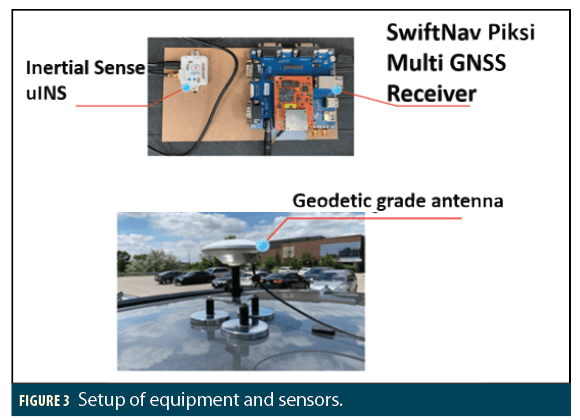
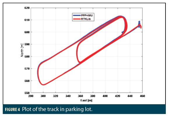
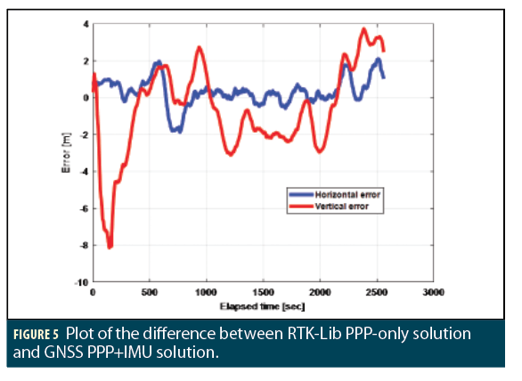
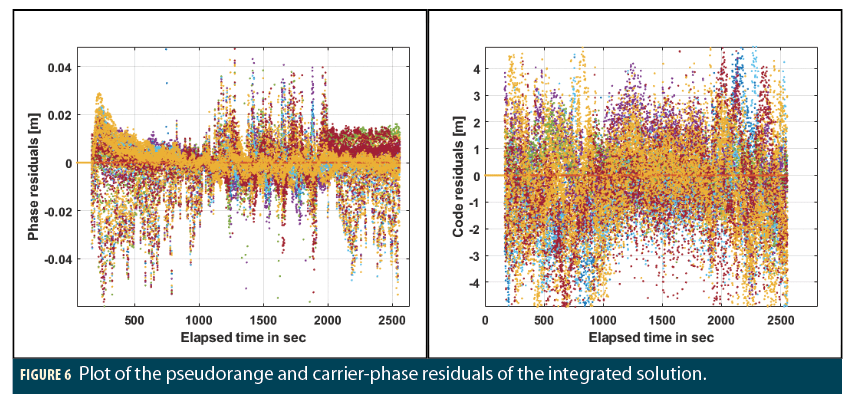
Figure 6 depicts code and phase residuals for the GNSS-PPP+MEMS IMU integrated solution of the parking lot data. Both code and phase residuals follow white-noise distributions. The code residuals mostly range from 5 m and the phase residuals range at the centimeter level. These orders of magnitude for the residuals are comparable to the ones with a PPP-only solution without any IMU integration. In the phase residuals, the portion where the vehicle is moving has slightly higher magnitude than the stationary part. This result can be improved by implementing zero velocity update (ZUPT) in the TC algorithm, which will be taken up in future work. The rms of the code residuals is 1.6 m and the rms for phase residuals is 4 cm.

Parking Lot Test With Outage

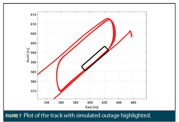
The real importance and value added by the IMU to the navigation system is realized only when there are not enough GNSS signals or during a GNSS signal outage. In this section, simulated outages for 30 seconds are performed and tested for the accuracy performance of the algorithm. During the outage, performance of the algorithm with just three-satellite and two-satellite availability is assessed. In Figure 7, a partially zoomed-in version of the track shown in Figure 4 is depicted to have a clear view of the simulated outage area. The portion of track highlighted in black is the area where simulated outages are performed.

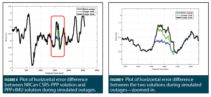
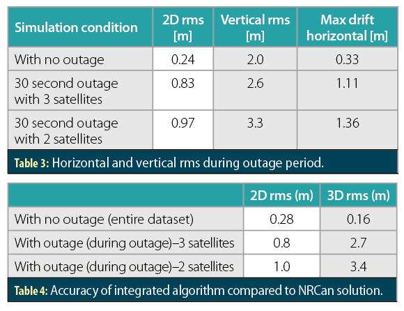
To indicate the performance accuracy of the algorithm, horizontal error compared against the NRCan CSRS-PPP is plotted in Figure 8. Here, the blue horizontal error is when there is no outage simulated. The green coloured horizontal error is when there are only three satellites available during the simulated outage. During the outage, the horizontal rms is 0.83 m and the maximum bias is 1.11 m. The black horizonal error in Figure 8 corresponds to the performance when there are only two satellites available during the simulated outage. During this outage, the horizontal rms is 0.97 m and the maximum bias is 1.36 m.

Figure 9 is a zoomed-in version of the plot of horizontal error discussed in Figure 8. After this outage, it takes a few seconds for the integrated solution to go back to the track with no outage simulated. This performance indicates that the lower the number of satellites during an outage, the lower the accuracy is. The accuracy drops steeply with the loss of each satellite.

Table 3 compares the statistics during the GNSS simulated outages in terms of horizontal and vertical rms. It is evident that when there are 2 or 3 satellites available to coast on, the solution still performs at the decimeter level of accuracy compared to the NRCan CSRS-PPP solution. Therefore, by using a low-cost, dual-frequency GNSS PPP with MEMS IMU, it performs at least 30% better than a single-frequency GNSS PPP with MEMS IMU, as demonstrated in a 2017 paper by Gao Z, Zhang H, Ge M, et al: A single-frequency GNSS PPP with MEMS IMU performed at meter-level accuracy, when there is an outage period of only 3 seconds.

Conclusions and future research

The navigation system of low-cost, dual-frequency GNSS-PPP solution tightly integrated with a MEMS IMU performed at the decimeter level of accuracy when there were no outages. A 30-second outage test showed that the algorithm performs with a rms error of 0.83 m in horizontal and 2.6 m in vertical directions, while there are three satellites available for the tightly-coupled solution to use. Whereas, when there are only two satellites during an outage, the horizontal rms is 0.97 m and vertical rms is 3.3 m. Table 4 gives an overview of the system’s performance accuracy with and without GNSS signal outage.

The tightly-coupled low-cost, dual-frequency GNSS-PPP and MEMS IMU performs with at least 30% better 2D rms when compared to low-cost, single-frequency and MEMS IMU integrated unit as examined in the 2017 research, using 3 second simulated GNSS measurement outages. The dual-frequency GNSS-PPP with MEMS IMU forms a complete low-cost solution with decimeter-level accuracy with respect to a GNSS-PPP reference solution. Such a navigation system can be used for many applications such as autonomous navigation, pedestrian dead reckoning, drones and other modern-day applications to improve accuracy and continuity of the navigation solution.

As part of future work, the algorithm will be tested in different challenging environments and different constraints. GNSS signal outage will be tested in environments such as tunnels, highway underpasses and downtown areas. To better estimate yaw angle while the vehicle is stationary, ZUPT will be implemented. Also, different scenarios such as performance of satellites from different constellations during an outage will be tested and assessed. Finally, to gain better vertical component results, vertical direction will be constrained and assessed for improvements.

Acknowledgments

Authors would like to thank Natural Sciences and Engineering Research (NSERC) and York University for providing funding for this research and German Research Centre for Geosciences (GFZ), International GNSS Services (IGS) and National Centre for Space Studies (CNES) for data.

This article is based on a paper that was originally presented at the Institute of Navigation GNSS+ 2019 conference in Miami, Florida.