GNSS Compare: Real-time Algorithms with Raw GNSS Measurement on Android Smartphones

An Android mobile application, GNSS Compare can provide a real-time position using Galileo and GPS dual frequencies. It directly logs data from the real-time algorithms, and the retrieved files are used for analysis.

While the principles of the analysis in this article of Android-derived code-based pseudoranges from a dual-frequency Xiaomi Mi8 smartphone focus on GPS, they also apply for Galileo. We investigate carrier-to-noise density ratios (C/N0), the noise power and/or other unmodelled effects in single-frequency pseudoranges (L1, L5) and in the ionosphere-free (IF)
combined ones by examining extended Kalman filter (EKF) innovation vectors.

The differences in terms of positioning performance of the EKF is shown when using solely the single-frequency pseudoranges from GPS L1, L5 signals and their IF combination. The results shown here are retrieved from the internal logged files by GNSS Compare; no additional post-procesing was done. This is one of the advantages of the application: the logging of low-level information that can then be visualized in any programming environment.

After describing the GNSS standard point positioning (SPP), we present the measurement models for GPS code pseudoranges together with the EKF estimator and its elements (e.g., dynamic model, process noise model). Finally, we present the test and experiment analysis carried out for a static user, and conclusions drawn from the results.

GNSS SPP Technique

The SPP technique involves use of the broadcast ephemeris together with a set of coefficients to determine satellite clock bias. Modelling of the signal propagation error sources (e.g., ionosphere, troposphere) is needed along with an estimator that solves the PVT problem (e.g., EKF).

For the retrieval of broadcast ephemeris and the satellite clock bias coefficients, GNSS Compare uses a Secure User Plane Location (SUPL) server provided by Google (supl.google.com:7276). The server can deliver this information for both GPS and Galileo constellations, given a connection to the internet. The server also supports GLONASS.

Measurement Model. To obtain the code-based pseudoranges from a smartphone with Android 7.0 version and upwards requires applying a set of algorithms to the raw parameters retrieved with the help of the application programming interface (API). These algorithms are described in the GNSS Compare’s website and with the code available on Github page and white paper cited in the Further Reading section. After the pseudoranges are computed, they can be described as:

where the superscript i indicates the ith satellite and the subscript j the frequency for each GNSS constellation (GPS L1 or L5); ρi is the geometric range between the receiver and the observed satellite; c is the speed of light in vacuum, δtR is the receiver clock bias and δtji is the satellite clock bias computed with the set of coefficients which are frequency dependent; dij,ion is the delay caused by the ionosphere and ditrop is the tropospheric delay; εji is the measurement noise, which in the absence of multipath and reduced effects of other unmodelled error sources (e.g., interference), is a zero mean gaussian distributed random variable. If we consider εji for multiple satellites as a vector (ε) then:

where R is the variance-covariance matrix of the measurement noise vector.

The term δtji should be computed using the clock coefficients from the Legacy Navigation Message (LNAV) message for single-frequency positioning with L1 and from the Civil Navigation Message (CNAV) for L5. For GPS we can only retrieve the LNAV, therefore we can’t distinguish the satellite clock coefficients from the SUPL server for L1 and L5. Considering this, in the present study, we access in the GPS-related processing the information contained only in the LNAV message for both L1 and L5.

Equation (1) is non-linear due to the geometric range ρi. The linearization can be done around a set of approximate coordinates (X0,Y0,Z0) of the user by applying a first-order Taylor series expansion. Therefore, the linearized expression of (1) is:

Where:

• yi is the difference between the measured and the predicted pseudorange measurement,

• represents the line of sight unit vector towards the ith satellite,

• δr=[ΔX,ΔY,ΔZ] is the vector containing the differences between the true and the approximate user position, differences that are regarded as unknowns in this situation.

For example, in the case of 4 observed GPS satellites (G), the linear measurement model can be written as the result of a matrix-vector multiplication:

In (4) the observation matrix (H) can be used in the presented form in a WLS or EKF as long as the receiver clock drift estimation is not of interest. If it is, then H should be modified by inserting an additional column of coefficients.

Extended Kalman Filter. The Kalman filter (KF) can fuse the information about how a system is evolving in time (according to a dynamic model) with the measurements made upon that system. The classic KF has two main requirements:

• the dynamic and measurement models to have uncorrelated gaussian distributed noises,

• the unknowns should be linked to the dynamic and measurement models in a linear form.

In the context of GNSS, the KF is a suitable choice for the estimation of the PVT. However, because the GNSS pseudorange measurements require linearization, an EKF was implemented to estimate the PVT. In this particular case, (1) is linearized, at each epoch, around the time predicted coordinates according to the chosen dynamic model. Further on we recall the EKF equations, describe the dynamic model for the states of interest (position and receiver clock) and the tunning of the filter.

Considering a linear relationship between the state vector (x) at epoch k and the dynamic model then we can write the time prediction and measurement update steps without the associated variance-covariance matrices (VCMs) as:

where the superscripts: ^ (hat) denotes an estimated quantity, the – (dash) represents the time prediction and the + (plus) the measurement update; Fk is the transition matrix; wk is the process noise [wk~N(0,Qk)], Kk is the Kalman Gain and γk is the innovation vector.

The innovation vector (γk)represents the difference between the pseudorange measurement and the predicited measurement using the information (about position and receiver clock bias) from the time predicted state vector. From a statistical point of view, γk is a zero mean gaussian random vector (ideal case) with a VCM [γk~N(0,Sk)] that contains both the contribution from the noises in the dynamic and measurement models. A more insightful view of the latter statement can be achieved by inspecting the expression of Sk:

In this equation the time predicted VCM of the state vector (Pk–) is being mapped in the measurement domain by the observation matrix (Hk) to which the VCM of the measurements (Rk) is added. For this reason γk is a useful parameter to analyze the performance of the EKF and the measurement quality at the same time.

Dynamic Model. Various dynamic models considered in the GNSS Compare’s implementation of the EKF (e.g., for vehicles, pedestrians). Here we focus on a static user, therefore we define our state vector, transition matrix and the VCM of the of the process noise to be:

where xpos, Fpos and Qpos were designed taking into account the user being static. Here we emphasize the approximation of Qclock:

• is the Power Spectral Density (PSD) of the white noise,

• is the PSD of the random walk of the frequency noise.

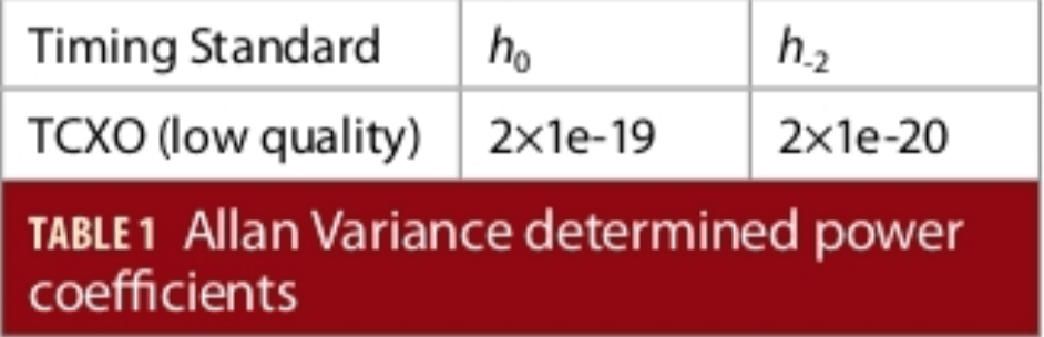
In (11) h0 is the power coefficient of the white noise and h-2 is the power coefficient of the random walk of the frequency noise. These parameters can be retrieved after performing an Allan Variance analysis for the receiver’s clock.

Tuning. The tuning process of the EKF involves the choice of values to be assigned in the R and Q matrices such that it best fits the real situation in the field. More explicitly, it means how much confidence we allocate to the measurements and to the dynamic model that will finally determine the performance of the EKF in estimating the PVT. We have implemented the form of R matrix which assumes no cross-correlations between satellites.

The values for the power coefficients h0 and h-2 correspond to a low quality temperature compensated crystal oscillator (TCXO) shown in Table 1, where the values are in units of seconds. Taking into account that the receiver clock states are expressed in units of meters, when h0 and h-2 are used to approximate (11), they should be converted in the same units by multiplying them with the square of speed of light.

The EKF and its tunning described above was implemented in the StaticExtendedKalmanFilter Java class described in the GitHub open-source code document. GNSS Compare has two other classes with EKFs designed and tuned for:

• PedestrianStaticExtendedKalman Filter,

• DynamicExtendedKalmanFilter.

The EKF for the dynamic user also includes the modelling of the velocity. The main principles for both classes do not differ from the static user case.

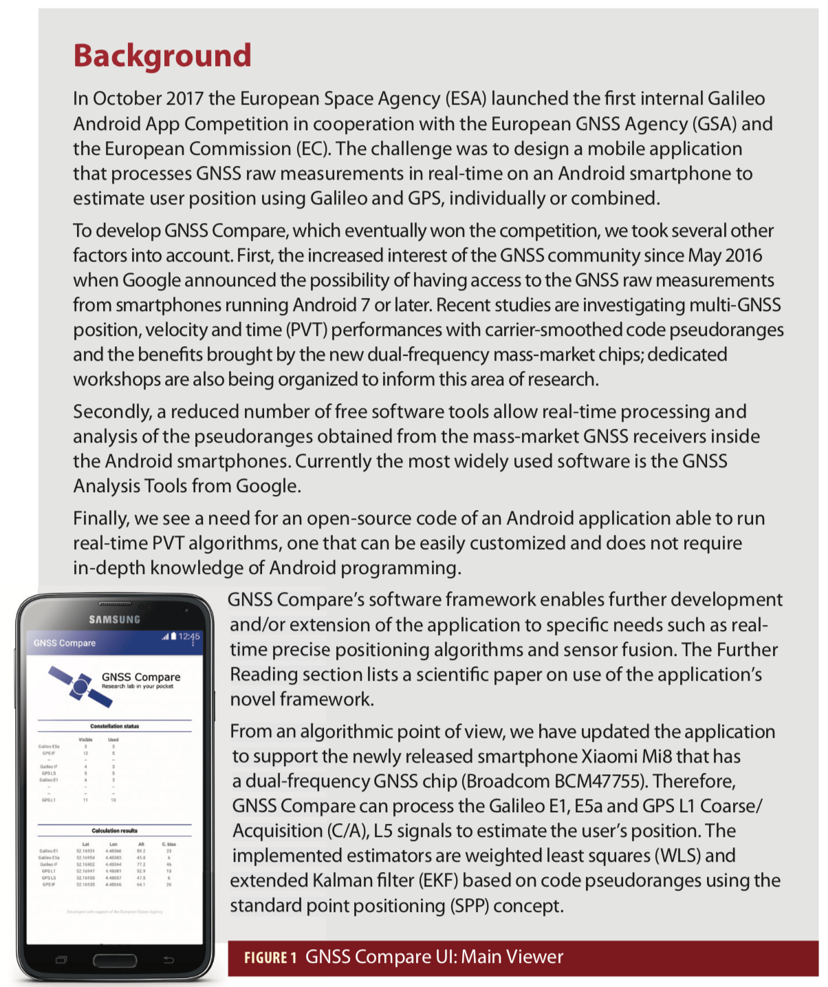
User Interface

Figure 1 shows the display that appears once the application is started. In the Constellation status part, the user can find information regarding the visible satellites, which signals are being tracked (e.g., Galileo E5a, GPS L5) and how many are used in the PVT estimation. By inspecting the Calculation results, one can monitor and analyze the real-time estimation results of the position (latitude, longitude, altitude) and of the receiver clock bias.

GNSS Compare offers the option to choose the PVT estimator that suits the situation in the field (e.g., static, dynamic) via the UI:

• Weighted Least Squares (WLS),

• Static EKF,

• Dynamic EKF,

• Pedestrian EKF.

The PVT estimator can be changed, for example, from WLS to Static EKF while the application is running. Such feature allows the user to test and validate algorithms and their tuning in real time.

More details about the GNSS Compare’s UI and how to access the different views can be found in the online documentation.

Test and Performance Assessments

A static test took place on the roof of the Navigation Laboratory of the European Space Research and Technology Centre (ESTEC) in Noordwijk, Netherlands. A Xiaomi Mi8 smartphone which has a dual-frequency GNSS chip (BCM47755) was placed near a reference point whose coordinates (latitude 52.218469, longitude 4.419383, height 58 m) were determined using real-time kinematic (RTK) techniques.

GNSS Compare was configured to use the GPS signals at 1 Hz for PVT estimation in real-time, in parallel, from L1, L5, IF combination of L1 and L5. For each configuration, the logging of the EKF’s output (innovation vector, receiver clock bias estimation, estimated position etc.) and other relevant information (satellite IDs, C/N0, pseudoranges, etc.) was enabled. Initialization of the EKFs was done using the position information provided by the Android Fine Location through the Android API.

The total duration of the test was approximately 15 minutes (900 seconds) starting at 8:35 a.m on 16 November 2018. That specific time window had a good availability and geometry of the GPS satellites transmitting both on L1 and L5. Twelve GPS satellites currently transmit on L1 and L5.

Performance Assessment. These results are plotted from the GNSS Compare logged files in the Github repository in the NAVITEC_loggedFiles folder. The archive within the folder contains the following text files:

• KalmanFilterFileLogger_GPS L1,

• KalmanFilterFileLogger_GPS L5,

• KalmanFilterFileLogger_GPS IF,

• RawMeasurementsFileLogger_rawMeasurements.

The last file has the Android GNSS raw parameters logged in the same format as Google’s GnssLogger App. It can be useful for post-processing and verification purposes.

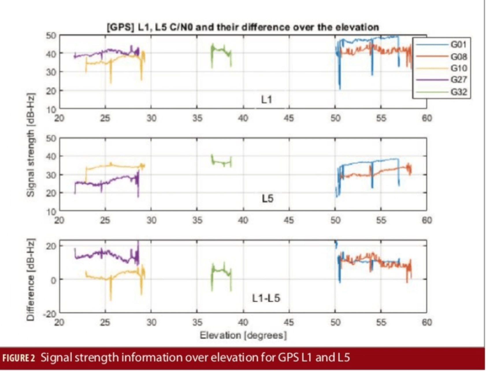
We begin the analysis by inspecting the C/N0 values for L1 and L5 from the following satellites: G01, G08, G10, G27 and G32.

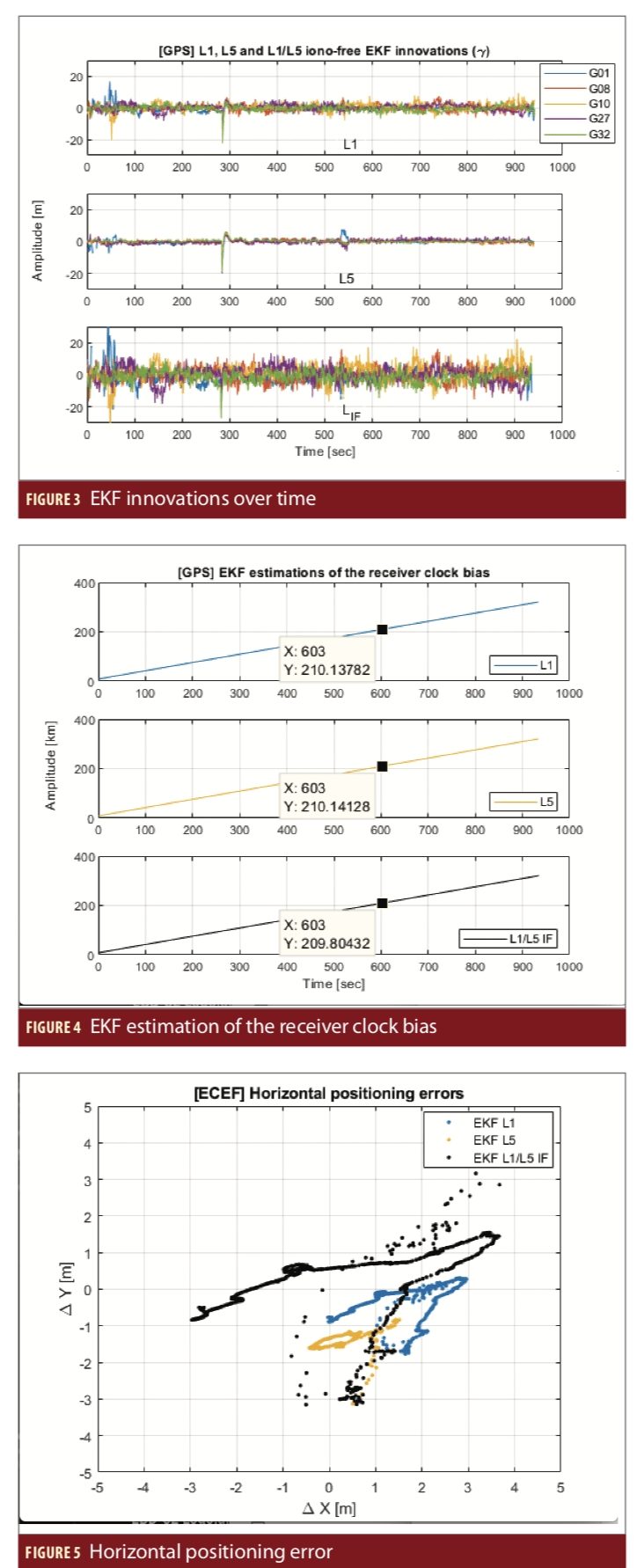
Figure 2 shows that there is a significant difference between the C/N0 values of L1 and L5. This behavior can be related to the fact that the design of a smartphone antenna able to capture also the L5 signals represents one of the main challenges.Even though the minimum transmit power of the GPS satellites is expected higher on L5 than L1, the power received by the smartphone on the L5 signals can be notably lower than the one seen on the same satellite but on the L1 signal.

Figure 4 shows over time the innovation vectors (γk) from the three EKFs that were processing the code-based pseudoranges from L1, L5 and L1/L5 IF combination in parallel. The GPS L1 signal has a binary phase shift keying (BPSK) modulation with a chipping rate of 1.023 MHz, often reprsented as BPSK(1). In the case of GPS L5, the same modulation technique is used however with a chipping rate that is 10 times higher than GPS L1, which can be written as BPSK(10). A higher chipping rate causes the PSD of the L5 signal to have a wider frequency occupation which also implies a narrower autocorellation function. These characteristics allow more accurate code tracking, better rejection of narrowband interference, increased robustness against multipath and improved signal accuracy.

The effect of the BPSK(1) and BPSK(10) can be visually observed, at the measurement level, in Figure 3. For L5 the innovations are lower in magnitude and variation when compared with the ones of L1. This means that the L5 code-based pseudoranges have a better quality.

Regarding the IF combination of L1 and L5, the obtained innovation vetors have the highest variance. The main gain of this linear combination is the removal of the first-order ionospheric delay up to 99.9%. However the variance of the noise of the IF combined pseudoranges is approximately more than five times higher than the original ones as seen in the equation below obtained by applying the propagation of uncertainty law:

The analysis on the effect of using different signal structures and the IF combination can be complemented with a numerical one. By computing the standard deviation of the innovations (σγ) presented in Figure 3, one can investigate the different measurement noise levels.

Table 2 shows that for this particular scenario, σγ,L1 is approximately 1.5 times higher than σγ,L5, on average. For the IF case, σγ,IF is roughly 2 times higher than σγ,L1 and nearly 3.5 times higher than σγ,L5. From this analysis an early expectation can be made in the sense that the best PVT performance is supposed to be given by the L5 only code-based positioning, followed by L1 and the L1/L5 IF combination.

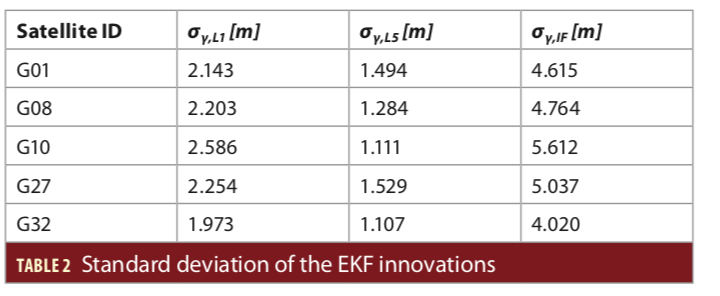
The next step in the analysis is to investigate the estimation of the receiver clock bias by the three EKFs.

In Figure 4 the receiver clock bias behavior is consistent between the presented cases. The bias reached a value around 210 km in 10 minutes, which means roughly a drift of 350 m/s. This is in line with the TCXO frequency stability of few parts per million (ppm). With such type of analysis is possible to form a good idea about the performances given by the internal receiver clock of the Xiaomi Mi8.

Taking into account that the measurement quality for the code-based pseudoranges from GPS L1, L5 and L1/L5 IF combination have been investigated along with the analysis of the receiver clock bias estimation, the discussion about the positioning performance can follow.

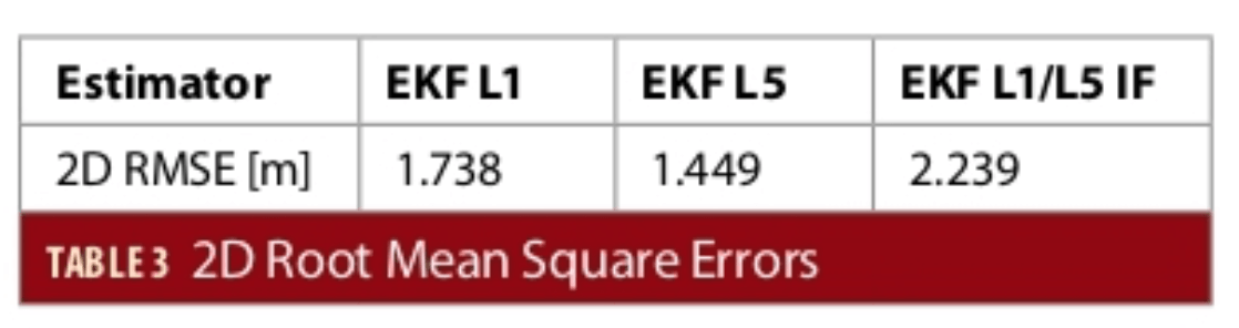
Figure 5 represents the error on X direction (ΔX) and Y (ΔY) direction, in the ECEF frame, of the estimated positions. The expectation formed from the analysis of the EKF innovations (Figure 3) is confirmed, in the sense that the best performance is given by the GPS L5 code-based pseudoranges followed by L1 and the L1/L5 IF.

The root mean square error (RMSE) measure quantifies the position estimation performances; see Table 3.

For this scenario, the L1/L5 IF combination gives the least performance even if the first-order ionosphere delay is removed up to 99.9% from the pseudoranges. When the ionosphere is less active (morning), the delays caused by it are not major, therefore the IF combination noise decreases the measurements quality (in the absence of other effects like multipath). The ionospheric delay from the L1 and L5 code-based pseudoranges was corrected with the Klobuchar model.

Conclusions

The design of the GNSS Compare Android application, its open-source code and online documentation address the issue of the reduced number of free tools for Android GNSS raw measurements processing in real-time. Analysis using measurements from a dual-frequency smartphone Xiaomi Mi8 processed retrieved code-based pseudoranges from GPS L1, L5 and their IF combination in three parallel EKFs, in real-time, to estimate the position of a static user. The output of the EKFs (innovation vector, receiver clock bias estimation, position estimation, etc.) was logged in files available online on GNSS Compare’s Github repository.

Several observations can be made:

• the utility of running multiple EKFs in real-time using different GNSS signals (GPS L1 and GPS L5),

• the effect of the GNSS signal structures (L1 compared to L5) in the EKF innovations,

• the measurement noise increase of the GPS L1/L5 IF combination,

• the horizontal positioning performance of the three EKFs.

GNSS Compare has received highly encouraging feedback from the communities represented by scientists and software developers. In 2018, the application won several prizes:

• 1st place at the first edition of Galileo Android App Competition organized by ESA

• 1st place at the 2018 European Satellite Navigation Competition (ESNC) Living Lab Prize

• 2nd at the 2018 ESNC Czech Republic Challenge.

These competitions also evaluated the business potential of the initiative. As of December 2019, GNSS Compare has more than 10,000 downloads.

Future Work

The analysis can be extended to Galileo E1 and E5a signals and the real-time algorithms (e.g., precise point positioning, sensor fusion). The software framework of the application can be used to investigate the advantages of sharing low-level GNSS data (atmospheric corrections, EKF innovations, etc.) between multiple users over the internet. The concept is similar to the one for Cooperative Intelligent Transportation Systems (C-ITS) and has the potential to improve the positioning accuracy, reliability, availability and robustness of GNSS in harsh environments such as urban areas.

Acknowledgment

The developers of GNSS Compare thank the ESA’s Directorate of Navigation and Directorate of Technology, Engineering and Quality for support throughout the development and improvement of GNSS Compare. We also highly appreciate ESA for promoting the application in the online press, social media and during ESTEC’s 2018 Open Days. As a result, GNSS Compare accumulated over 3,000 downloads.

Further appreciation is given to these ESA employees who have shared their knowledge and experiences with us: Paolo Crosta, Nityaporn Sirikan, Gaetano Galluzzo, Paolo Zoccarato, and Tim Watterton. Finally, special thanks to Matej Poliacek and Peter Vanik from the ChocolaTeam, who have trusted the framework we’ve developed and are using it as the calculation back-end of their application.

Authors

Sebastian Ciuban is a GNSS Engineer in the Space Department of CGI Nederland B.V. where he focuses on signal processing algorithm design activities for a snapshot receiver within the project called Secure Tracking Services (S-TrackS). He received his MSc. in Aerospace Systems–Navigation and Telecommunications from École Nationale de L’Aviation Civile.

Mateusz Krainski currently works for Showmax, where he’s responsible for the development of the internal Content Management System and a number of microservices. Previously, he designed and implemented the software architecture for GNSS Compare while an engineer at the European Space Agency.

Dominika Perz is a software and control engineer who obtained her Masters degree in control engineering and robotics at Wroclaw University of Science and Technology. As an ESA Young Graduate Trainee in the Guidance, Navigation and Control team, she focused on developing a simulation tool for final stage of lunar landing.