
Research has focused on methods to analytically determine bounding probability distributions and parameters and identify the conditions under which such bounds are guaranteed to hold. This column summarizes several important examples from this research to highlight the most useful principles and techniques.
The GNSS Solutions column in the May/June issue of Inside GNSS ([1], hereafter “Part I”) explained that error bounds valid to very low probabilities such as 10-7 to 10-9 are needed to calculate protection levels (PLs) that can be compared to safe error limits (“alert limits”) to confirm that safety is maintained in real time. It also highlighted the difficulties in creating such error bounds when the probability distributions governing GNSS errors at such small probabilities are unknown and often have tails that are fatter than those of a normal (Gaussian) distribution.
Part I addressed this problem empirically by showing how Gaussian distributions with larger (inflated) sigma values can be used to bound the tails of sampled error data. This approach is commonly used and provides some confidence that rare-event error values used to compute protection levels for GNSS applications with demanding integrity requirements are acceptably conservative. However, when inflated sigma values are determined empirically, no guarantee exists that the resulting position-domain protection levels bound actual errors to the required probabilities.
To address this problem and to further fortify the confidence that safety-of-life users have in their protection levels, a significant amount of research has focused on methods to analytically determine bounding probability distributions and parameters and identify the conditions under which such bounds are guaranteed to hold. While none of these magically solve the problem of not knowing the true error distributions, they provide a great deal of insight into why this problem is hard and what can be done to reduce bounding uncertainty without requiring extreme conservatism (e.g., very large inflation factors, which result in loss of availability). This column summarizes several important examples from this research to highlight the most useful principles and techniques.
CDF Bounding
A paper published by Bruce DeCleene in 2000 [2] was a key starting point in understanding the difficulty of analytically bounding rare-event errors and proposing analysis techniques. This paper explained the concept of cumulative distribution function (CDF) bounding that is the foundation for most practical bounding techniques. CDF bounding requires that the CDF of a bounding distribution (in the range domain) exceed the true (unknown) CDF for every error value above the mean error and be below the true CDF for every error value below the mean. When multiple statistically independent bounding distributions in the range domain are combined (convolved) together to form position-domain error distributions, the resulting distributions will also bound actual position-domain errors as long as the following conditions are met for both the bounding distribution and the underlying error distribution [2,3]:
• Both distributions are zero-mean (or any non-zero means are known and accounted for in determining error probabilities).
• Both distributions are symmetric about the mean, meaning that the shape of the probability density function (PDF) and CDF on both sides of the mean are identical. Symmetric distributions have the same mean, median, and mode.
• Both distributions are unimodal, meaning that the distribution has only one peak frequency of occurrence and continuously falls off in probability on both sides of this peak (i.e., its PDF has only one “hump”).
In practice, the bounding distribution is usually a Gaussian distribution with a standard deviation made large enough to bound data sets of actual error samples (the empirical technique in Part I uses this approach). This supports the existing Gaussian formulation of the protection level equations for civil aviation applications and makes range to position domain convolution straightforward.
The difficulty, of course, is determining if these properties hold for an unknown actual error distribution. In practice, even for symmetrical distributions, the true mean error is difficult to observe with sufficient confidence, so a conservative estimate of it needs to be included in the inflated bounding sigma. In addition, error distributions are not symmetric and unimodal in general, especially for low-probability errors. Some GNSS range-domain error sources, such as multipath and atmospheric delay, may have different distribution shapes on positive and negative sides for physical reasons. Also, multiple local maxima often occur at low probabilities in actual data, but it is hard to tell if these are due to statistical randomness or actual error behavior. As noted in Part I, the “nominal” conditions described by a single error distribution encompass many different nominal, near-nominal, and off-nominal conditions. Off-nominal events with low probabilities can be bounded by a single distribution with an inflated CDF, but they can create additional “peaks” in the PDF that violate the unimodal condition.
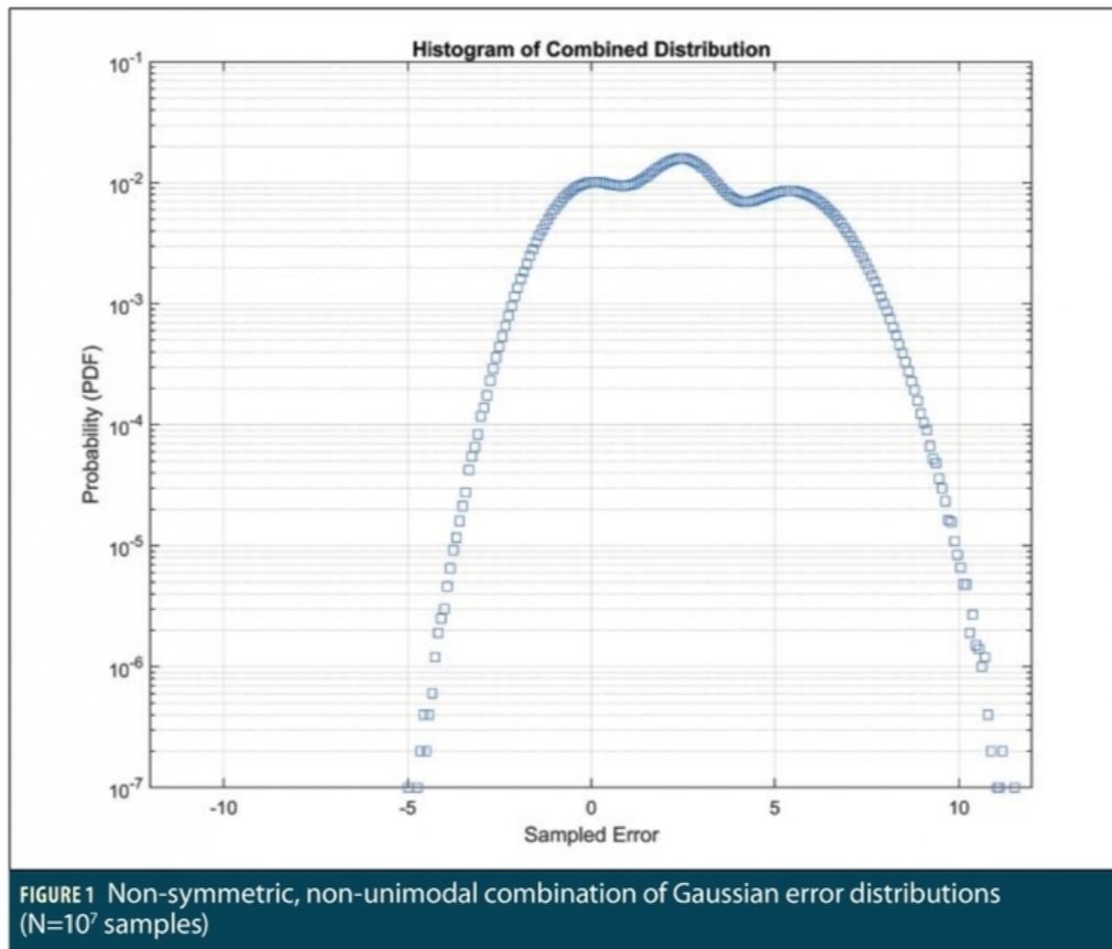
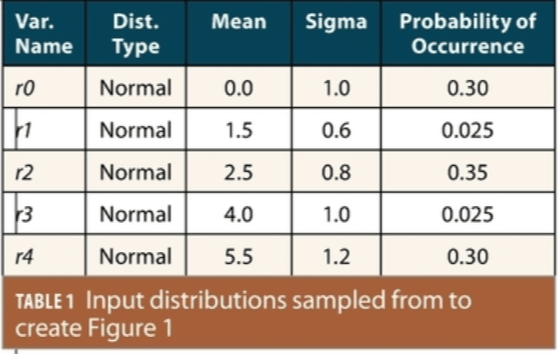
For illustration, Figure 1 shows the histogram (in PDF form) of a data set generated by Monte Carlo sampling from multiple Gaussian distributions with different means in the manner conducted in Part I. Table 1 shows the five Gaussian distributions sampled from and the probability that applies to each, meaning that each of the 10 million samples collected has that probability of being taken from the corresponding Gaussian distribution. Since four of the five distributions (all but r0) are biased in the positive direction by different amounts, the resulting distribution is not symmetric. In addition, because two of these distributions (r2 and r4, with means of 2.5 and 5.5, respectively) have similar probabilities of occurrence as the unbiased distribution, two humps appear at those bias values and prevent unimodality (with the hump from r2 being the highest).
Paired Bounding and Extensions
Given how difficult it is to guarantee CDF bounding by proving that the above conditions are met, subsequent work developed approaches for achieving a similar guarantee while relaxing them. One such approach is “paired bounding” as described in [3]. This approach replaces the single bounding distribution of [2] with a pair of distributions, one which “left bounds” all possible error values and another which “right bounds” all error values. Mathematically, defining GL and GR as the CDFs of the left and right bounding distributions, Ga as the unknown actual CDF, and x representing the vector of possible error values, this requires [3]:
A combination of left and right-hand bounding distributions that satisfies these conditions preserves bounding through convolution (including range-to-position domain convolution) even if these three distributions do not meet the (single) CDF bounding conditions described above.
One difficulty of this approach is the need to create and convey distinct left and right-hand bounding distributions to users whose protection-level equations assume a single bounding distribution. The implementation proposed in [3] creates separate but parallel left and right-hand Gaussian bounding distributions with the same standard deviation and the same bias magnitude as the empirical distribution used as input (i.e., a data-generated estimate of the actual distribution). Thus, only a single bias parameter is added to the standard deviation that is already transmitted. If existing user interfaces do not have room to add this bias, the broadcast standard deviation must be inflated substantially to bound this bias with a zero-mean Gaussian distribution.
Another weakness of paired bounding is illustrated in a more recent paper [4]. It is very difficult to meet the pair-bounding condition when, as just mentioned, the actual distribution (Ga) is represented by an empirical function generated from data (e.g., a histogram of error values collected into discrete bins) without excessive conservatism, such as selecting a bias value that is orders of magnitude larger than the sample mean. An extension of paired bounding using “excess mass” functions (see [5]) is one way to ameliorate this conservatism and is also applied in [4].
Single-CDF and Paired Bounding
The method proposed in [4] combines the single CDF and paired bounding techniques in a two-step process. The first step applies a heuristic algorithm to create a single discrete symmetric and unimodal distribution from the original data set (expressed as a histogram) which in general is neither symmetric nor unimodal. The second step determines the means and standard deviations of two Gaussian distributions that left-bound and right-bound the output of the first step. Because each of these two bounds starts with a symmetric, unimodal distribution but only has to bound half of its CDF (instead of all of it), the resulting bias needed to meet the CDF bounding condition is much lower than for single-step paired bounding. Matlab scripts that implement the methods described in [4] are available online at [7].
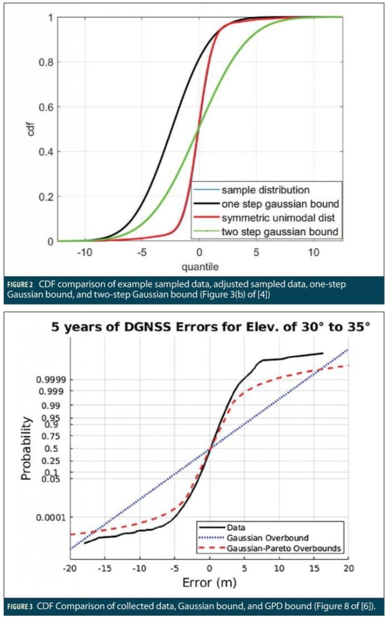
Figure 2 (from Figure 3(b) of [4]) shows this improvement graphically by comparing the CDFs of the tighter two-step Gaussian bound (in green) to the looser (more conservative) one-step Gaussian bound that would have been generated (in black) using paired bounding only. The blue line represents the CDF of the original sampled data, and the almost identical red line shows the CDF after heuristic modification to make it symmetric and unimodal.
Non-Gaussian Bounding and EVT
The methods described above focus on developing Gaussian distribution bounds for empirical error data with unknown distributions. In other words, the only knowledge of the actual error distribution (at least in the tails) comes from the collected data itself. Many examples of collected error data have tails that appear fatter than Gaussian as far as the data extends. Any form of Gaussian bounding implicitly assumes that actual error probabilities beyond those covered by the number of samples (and are thus unobservable) fall below the Gaussian tail shape, which is very optimistic since Gaussian tails fall off quickly with increasing error sizes. Even within the range of probabilities covered by the empirical data, high inflation factors are often required to bound the observed tails (see the example in Part I).
Approaches have been developed that addresses this limitation by proposing non-Gaussian (and fatter-than-Gaussian) distributions to bound the tails of the distribution. The method proposed in [6] combines Gaussian bounding of the core (center) of the actual error distribution with bounding via a generalized Pareto distribution (GPD) for the tails. Use of the GPD is motivated by Extreme Value Theory (EVT), which has been applied in many fields to approximate bounds on low-probability events. EVT states that the tails of all continuous distributions approach that of the GPD as the threshold separating the tail from the core approaches a maximum value (up to infinity—see Section 3 of [6] for details). Since the actual threshold cannot be infinite to be useful, this is an approximation at best, but the GPD is practically useful as a better model of fatter-than Gaussian tails. Section 4 of [6] describes a method of selecting appropriate threshold values and estimating the Gaussian and GPD parameters of the core and tail components that form a combined bounding distribution.
The benefits of the combined Gaussian core/GPD tail bounding approach in [6] is illustrated in Figure 3 (Figure 8 from [6]), which uses a data set of 5 years of estimated Differential GPS pseudorange errors between two NGS CORS reference stations tracking satellites at elevation angles between 30 and 35 degrees (range-domain errors are a function of elevation angle, so only measurements at nearly the same elevation angles should be combined to limit the “mixing” phenomenon described in Part I). In this figure, the y-axis probabilities are scaled such that the CDF of a Gaussian distribution is a straight line. The black line shows the empirical CDF of the observed data, which is much more closely fit by the combined Gaussian/GPD bounding CDF (dashed red line) compared to the dotted blue line formed by a single bounding Gaussian distribution. As a result, use of the Gaussian/GPD bound in (modified) protection-level calculations gives a lower protection level than would be obtained using existing protection level equations with a single Gaussian distribution.
Conclusions
This article has introduced several analytical approaches to bounding unknown GNSS range-domain error distributions with Gaussian distributions, potentially augmented with non-Gaussian tail distributions. Analytical methods have three general advantages over the purely empirical approach of Part I:
• They provide additional flexibility in modeling low-probability (tail) error behavior,
• They are more systematic and repeatable, and
• They provide theoretical assurance that the resulting bounds hold at the required integrity probabilities under certain conditions.
In practice, these advantages are useful but are less important than they might seem. The use of non-Gaussian models of errors in the tail leads to significantly tighter bounds, but it conflicts with the many existing applications whose protection level equations assume Gaussian-distributed tails only. Systematized algorithms help reduce variations due to individual judgement, but extensive judgment is still required, particularly when deciding how to collect representative error data, how to sort it into sets that represent different environmental conditions, and how much error data is needed to provide sufficient sampling of errors at low probabilities.
Finally, the theoretical bases for assured bounds generally do not apply in the real world (or, at least, they cannot be demonstrated to apply), thus they can only be assumed or “asserted.” Beyond the conditions described here, these analytical methods (and the empirical approach in Part I) assume that range-domain errors on individual satellites are statistically independent when they are combined into the position domain. This is virtually never true due to atmospheric delays being correlated in space and multipath errors being correlated by the local reflective environment. Furthermore, all these methods assume that the empirical CDFs of collected error data are perfect models of the actual error distribution out to infinitely small probabilities. Because of practical limits on the number of data samples and unavoidable differences between practical data-collection scenarios and the much larger set of environments that affect actual users, this cannot be the case either. All these factors must be kept in mind when utilizing the results of any error bounding algorithm in a safety-critical application.
References
(1) S. Pullen, “Why is bounding GNSS errors under rare or anomalous conditions important?” Inside GNSS, May/June 2020.
(2) B. DeCleene, “Defining Pseudorange Integrity—Overbounding,” Proceedings of ION GPS 2000, Salt Lake City, UT, 2000.
(3) J. Rife, S. Pullen, P. Enge, B. Pervan, “Paired Overbounding for Nonideal LAAS and WAAS Error Distributions,” IEEE Transactions on Aerospace and Electronic Systems, Vol. 42, No. 4, October 2006..
(4) J. Blanch, T. Walter, P. Enge, “Gaussian Bounds of Sample Distributions for Integrity Analysis,” ibid, Vol. 55, No. 4, October 2018.
(5) J. Rife, T. Walter, J. Blanch, “Overbounding SBAS and GBAS Error Distributions with Excess-Mass Functions,” Proceedings of 2004 International Symposium on GNSS/GPS, 2004.
(6) J.D. Larson, D. Gebre-Egziabher, J. Rife, “Gaussian-Pareto Overbounding of DGNSS Pseudoranges from CORS,” Navigation: Journal of the Institute of Navigation, Vol. 66, No. 1, Spring 2019, pp. 139-150.
(7) “Gaussian Overbound,” Stanford GPS Lab Software Tools (Online), https://gps.stanford.edu/resources/software-tools/gaussian-overbound.


