
Estimating and quantifying errors in GNSS and other navigation user equipment is a common task and is important for understanding what roles or missions a given device is suitable for. Most users are familiar with the concept of accuracy, which is usually expressed as a bound on navigation error (relative to unknown truth) at a probability level between 0.5 and 0.95. This article expands on the concept of accuracy to estimate error bounds that are only violated with far smaller probabilities.
These bounds are required to calculate protection level equations that are used to verify navigation integrity in real-time for applications with very strict safety requirements. Protection levels are compared to limits on the maximum safe errors (“alert limits”) to confirm that safety is maintained for the current operation. Because much less is known about GNSS errors at the very low probabilities that apply to protection levels (e.g., 10-7 to 10-9), it is very difficult to extrapolate accuracy numbers to these low probabilities.
The starting point for understanding error bounding at different probabilities is the common use of the standard normal (or Gaussian) distribution to represent random errors. This is a normal distribution with a mean of zero and a variance of 1, meaning that its standard deviation or “sigma”, which is the square root of the variance, is also 1. Any normal distribution with a different mean and/or variance can be converted to a standard normal distribution simply by subtracting out the non-zero mean and dividing the variance by itself, then keeping track of these “normalizing” factors to convert back when needed.
The normal distribution is often used to model errors because of its simplicity, its convenience when combining multiple normally-distributed errors, and because of the Central Limit Theorem (CLT) in statistics, which states that the sum of n independent and identically distributed random variables approaches a normal distribution as n  ∞ [1]. Normal distributions with estimated means and variances generally give a reasonable model of at least 90% to 95% of observed errors, but the limitations of the CLT make this untrue at much lower probabilities.
Accuracy Statistics
To use the normal distribution to estimate accuracy, mean and variance (or sigma) values can be derived from theoretical considerations, but it is more common to generate them from the statistics of measured errors compared to known truth values. The following standard equations show how to calculate the sample mean ( ) and the unbiased sample variance (
 ) of a set of n measured error data points xi (i = 1,2, …, n) [2,3]:


For a well-calibrated system, will be close to zero and will be small compared to  , thus it can often be ignored or included in the “root-mean-square” or rms, where rms2 =
  .
.
Typical means by which accuracy is specified include Circular or Spherical Error Probable (CEP or SEP), which bounds 50% of 2-D or 3-D position errors; one-sigma or one-rms, which bounds approximately 68.3% of range or position errors if the errors are normally distributed; and 95th-percentile error bounds, which are equivalent to approximately twice the sigma of normally-distributed errors with zero or near-zero means (the actual normal distribution multipliers are ± 1.96 for 95% bounds, which cover the 2.5th to 97.5th percentiles, and ± 2.81 for 99% bounds, which cover the 0.5th to 99.5th percentiles). The 50th-percentile bounds for CEP and SEP are commonly determined directly by sorting the original data vector xi from low to high and reading off the midpoint values, but if a normal distribution is fitted, the 50th-percentile confidence interval multipliers are ± 0.675.
Protection Level Equations and Challenges
The statistical concepts used for accuracy also form the basis for developing protection level equations, but the context is quite different. As noted above, protection levels represent error bounds that can only be violated at the very small probabilities tied to the requirements of safety-critical GNSS applications. At these small probabilities, the assumptions and properties that apply most of the time break down, so extra precautions must be taken.
The standard form of protection level equation bounding nominal errors (conditions without significant faults or other anomalies) is as follows (shown here for the vertical dimension):

where the term surrounded by the square root sign converts range domain fault-free (assuming zero mean) error variances for each usable satellite i from 1 to n  to vertical position domain variances by multiplying each one by the appropriate squared entry of the weighted pseudo-inverse of the geometry matrix (
 ) (see [4]). The multiplier Kv,ffmd extrapolates the resulting one-sigma vertical position error to the required bounding value determined by the integrity requirement for the operation being conducted. For example, as in Satellite-based Augmentation Systems (SBAS), if VPL must bound nominal vertical errors to a probability of violation of 10-7 per operation, Kv,ffmd is 5.33 based on extrapolating the standard normal distribution to this extent [4]. In other words, despite the great difference between bounding probabilities of 95% or 99%, which can readily be observed with enough samples, and 1 – 10-7, which generally cannot, the mathematical formulation is the same. While other protection level expressions bound faulted conditions and include separate bias terms representing worst-case fault effects, SBAS protection levels use only the nominal formulation of (3) and require all possible undetected faults to be bounded by it.
Experience has shown that, while normal-distribution extrapolations to as far as 3 standard deviations (bounding about 99.7% of errors) are often justified, extrapolations beyond that typically fail. The reasons are numerous. Actual GNSS errors are generated by different physical manifestations, severities, and time evolutions of satellite, multipath, and atmospheric errors; thus they meet neither the independent nor the identically distributed assumptions of the Central Limit Theorem. The Central Limit Theorem does not apply to non-independent and non-identically distributed inputs, but it does suggest that distribution of such measurements will trend toward normal as the number of measurements gets very large. This effect is usually visible in the “core” of the distribution of measurements (e.g., within 95th or 99th percentiles) but less so for the few points outside these ranges.
Even if all input measurements are themselves independent and normally distributed, the impact of “mixing” inputs with different variances among the population was understood as far back as the mid-1960’s to create non-normal behavior. In fact, the combined distribution trends toward exponential for large deviations from zero, meaning that large errors become much more probable than would be predicted by the tails of a normal distribution with a single variance [5]. This has been observed with real data known to combine data with different variances (such as multipath from different directions with different reflecting surfaces).
Empirical Solution
The fundamental problem with rare-event error bounding comes from the fact that the tails of the actual error distributions are unknown but are known to at least be fatter (worse) than normal in most cases, yet the protection levels calculated for safety-of-life applications are based upon normal tails. This situation came about because, absent specific knowledge that another distribution provided a better fit, the normal distribution was the most natural one to base protection levels on. Since equation (3) or variants of it are standardized for use, the only approach to protecting against fatter-than-normal tails is to increase (“inflate”) one or more of the parameters in the equation to cover for the effects of these tails. In most cases, the range-domain error variances ( ) are inflated to accomplish this.
If there are no constraints on the actual error distributions, it is impossible to guarantee that any particular inflated value of  will bound the actual tail behavior. This leads to two different approaches. The empirical approach described below is simpler and more common. A later column will discuss more advanced theoretical approaches which attempt to take advantage of physical or other knowledge about actual error distributions.
Numerical Example
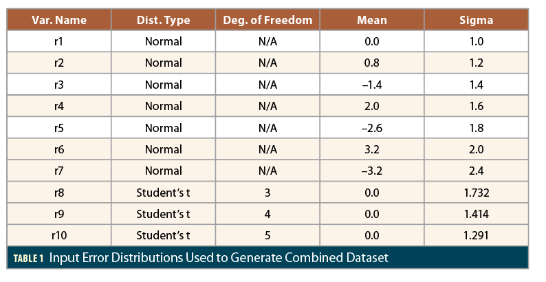
To illustrate the differences between accuracy and integrity bounding along with the empirical approach to deriving sigma inflation factors, a numerical simulation is shown here using Matlab to generate millions of samples of errors that are mostly normally distributed but suffer from the “mixing” of different distributions mentioned above. In this simulation, a total of 10 million random samples R were created by generating 1 million samples each from the 10 different error distributions r1, …, r10 shown in Table 1. Note that non-zero but offsetting (some positive, some negative) means are included, and three of the 10 distributions are non-normal “Student’s t” distributions with zero mean but fatter-than-normal tails [6].
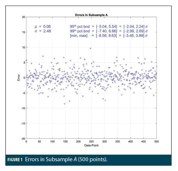
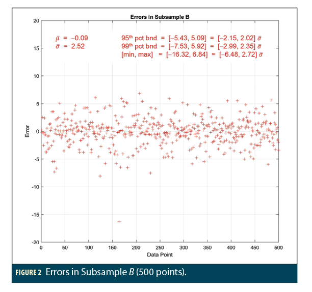
Figures 1, 2, and 3 show the results of three separate random subsamples A, B, and C, each containing 500 points from among the 10 million samples in the overall dataset R. The sample error mean, error sigma, minimum and maximum error, and upper and lower bounds at the 95th and 99th percentiles are shown on each plot along with the ratios of these quantities over the sample error sigma. For comparison, recall that the normal distribution sigma multipliers are ± 1.96 for 95% bounds, ± 2.81 for 99% bounds, and ± 3.09 for 99.8% bounds, corresponding to the minimum and maximum of 500 samples.
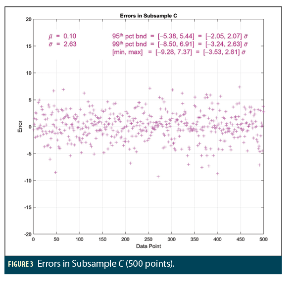
All three subsamples appear generally similar and show errors that appear to conform to what would be expected from normal distributions with the computed sample error sigmas. This is most true of subsample A in Figure 1, where no significant outliers appear, and the sigma multipliers that apply to the 95th, 99th, and min/max values are not far from the expected values but begin to exceed them in the tails. Subsample C in Figure 3 is similar except for the presence of multiple large negative errors (slightly beyond  ) that might suggest a trend toward non-normal tails in that direction. Subsample B in Figure 2 looks as well-behaved as subsample A with the single exception of the very large (
 ) negative error observed in a single data point. Oddities like these are often treated as “outliers” and neglected, but in this case, that single point hints at the severely fatter-than normal tails that would be clearly visible if a very large set of samples of the underlying distribution (or combination of distributions) were available.
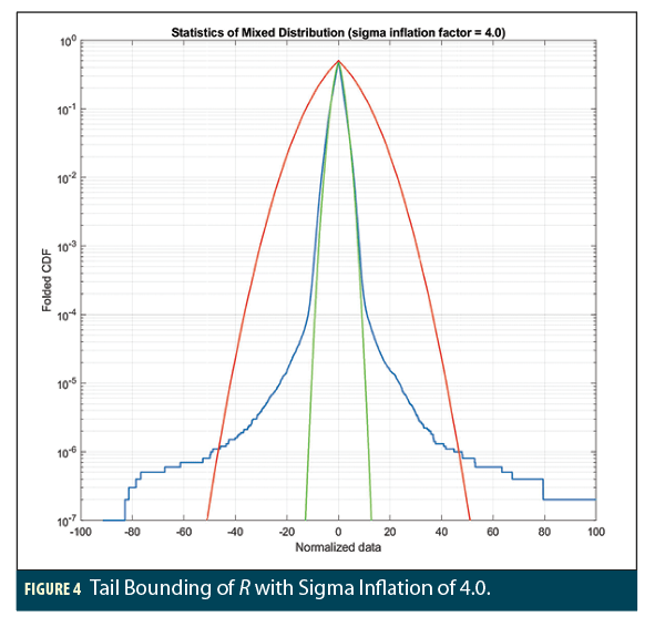
Of course, in this numerical experiment, all 10 million points comprising R are available and are plotted in the form of a “folded cumulative distribution function (CDF)” in Figures 4 and 5. A folded CDF plot is a two-sided CDF in which the probability of exceeding the absolute value on the x-axis in the same direction (either further positive or further negative) is shown (in semilog form in this case) on the y-axis. The actual distribution of the data in R is plotted in blue in Figures 4 and 5, and the CDF of a normal distribution with zero mean and the sample sigma is plotted in green (the actual sample mean and sigma of R are  and
and  ).
).
What is clear in both figures is that the normal distribution based on the sample sigma falls far short of representing the behavior of the actual data in R below a probability of about 0.01. Below 10-4, the actual tail behavior diverges greatly from the normal distribution. As explained above, this is not a surprising result. If the designers of safety-critical systems knew or could approximate that R was created by the mixture of 10 distributions shown in Table 1, a tailored bounding solution based on this knowledge could be created, but such knowledge is almost always absent (or is at least sufficiently uncertain). Given this, and given the fact that protection level bounding the actual data must be based on a normal extrapolation as in equation (3), the empirical approach mostly trusts that the available data composing R (that which can be plotted and assessed) is a full representation of the real uncertainty and then determines (by trial and error) the degree of sigma inflation (e.g., the multiplier to be applied to  ) that is sufficient to bound the plotted data to the required probability.
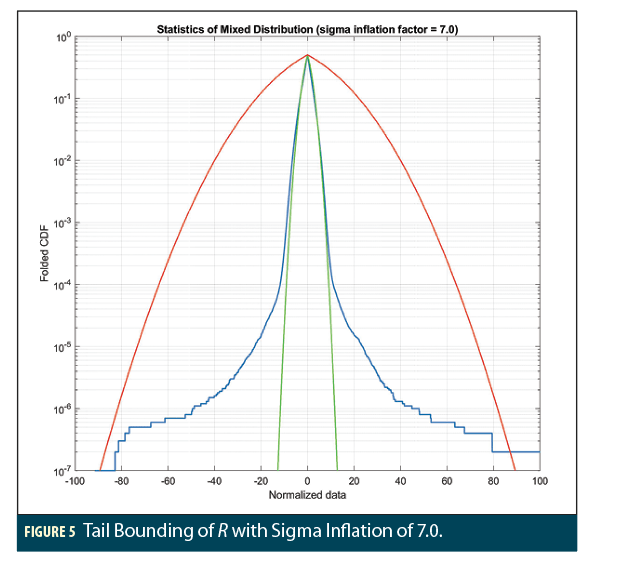
The only thing that distinguishes Figures 4 and 5 is the degree of sigma inflation applied to create the red curve. In Figure 4, the red curve represents a zero-mean normal distribution with an inflated standard deviation ( ) of 4 times the sample sigma ( = 4.0 = 9.92). The difference between the red and green curves is clearly visible, and the red curve appears to bound the actual error distribution down to a little below 2 × 10⁻⁶. If this probability satisfies the integrity bounding requirement, this inflation factor would be acceptable, but in most cases, a probability at or below 10-7 is required. Figure 5 shows how such a small probability can be achieved in this case if the sigma inflation factor is increased to 7.0 ( = 7.0 = 17.185). Even here, it is not clear if positive errors are bounded to this probability because R includes two errors (out of 10 million) exceeding 100.
While this degree of inflation is larger than what is typically required, this numerical example points out the difficulty of using nominal statistics based on hundreds or even thousands of independent samples to try to bound errors at probabilities of 10-5 and below. Fat tails (when compared to normal distributions) are commonly present and should be assumed to exist absent strong theoretical and statistical evidence to the contrary. However, when they are present, large sigma inflation factors will likely degrade system performance and availability. The analytical error bounding methods to be described in a future column are specifically focused on applying system-specific knowledge and statistical theory to lower the required inflation where possible. 
Useful Internet Links
(numbered references):
(1) “Central limit theorem,” Wikipedia, accessed 4/15/20. https://en.wikipedia.org/wiki/Central_limit_theorem
(2) “Sample mean and covariance,” Wikipedia, accessed 4/15/20. https://en.wikipedia.org/wiki/Sample_mean_and_covariance
(3) “Sample variance,” Wikipedia, accessed 4/15/20. https://en.wikipedia.org/wiki/Variance#Sample_variance
(4) Minimum Operational Performance Standards (MOPS) for Global Positioning System/Wide Area Augmentation System Airborne Equipment. Washington, DC, RTCA, DO-229E, December 2016.
(5) J. B. Parker, “The Exponential Integral Frequency Distribution,” The Journal of Navigation, Vol, 19, No. 4, October 1966. https://doi.org/10.1017/S0373463300047664
(6) “Student’s t-distribution,” Wikipedia, accessed 4/16/20. https://en.wikipedia.org/wiki/Student%27s_t-distribution


