A 4D extension of complex numbers, bicomplex numbers allow for a compact representation of GNSS meta-signals with components from two different frequencies. Acquisition and tracking algorithms are obtained from the bicomplex signal representation, giving it potential for effective dual-frequency GNSS signal processing.
DANIELE BORIO, EUROPEAN COMMISSION, JOINT RESEARCH CENTRE (JRC)
The effective processing of advanced Global Navigation Satellite System (GNSS) modulations, such as the Alternative Binary Offset Carrier (AltBOC) and Asymmetric Constant-Envelope Binary Offset Carrier (ACE-BOC), requires algorithms able to efficiently combine signal components from different frequencies. This also applies to GNSS meta-signals that are obtained by considering signals from different frequencies as a single entity.
In addition to properly combining different signals, these algorithms need to deal with measurement ambiguities, which may arise in the final pseudoranges generated from the composite correlation function. More specifically, the correlation function of a GNSS meta-signal may have secondary peaks and a false lock on such peaks may cause measurement ambiguities. While effective approaches to avoid this problem are available, they often require convoluted notations for the representation of the different signals and correlation outputs.
In standard GNSS signal processing, the use of complex numbers proved beneficial with respect to real numbers, leading to compact notations and often to more revealing signal and correlation representations. For instance, correlator outputs can be effectively represented as a single complex number rather than two real components. The polar representation of a complex number is used to isolate the residual correlator phase error, which is minimized in Phase Lock Loops (PLLs). Moreover, complex exponentials effectively represent 2D rotations and simplify algorithm development.
There are several multi-dimensional extensions of complex numbers that have been introduced to effectively represent multi-component signals and simplify algorithm development. The most well-known of such extensions is the set of quaternions, a 4D generalization of complex numbers with three imaginary units. In strapdown inertial navigation, quaternions have led to numerically stable and efficient navigation algorithms. More recently, the set of dual-quaternions, an eight dimensional real algebra, has been adopted to represent rigid motions in 3D spaces with applications in robotics, kinematics and computer vision. These extensions are usually denoted as hypercomplex numbers.
This article investigates the potential of the set of bicomplex numbers for the representation and processing of GNSS advanced modulations and meta-signals. Bicomplex numbers are a 4D extension of complex numbers with a commutative product. They can represent two GNSS signals from two different frequencies as a single quantity leading to a compact notation for effective algorithm development. Bicomplex numbers also can be used for the representation of composite correlator outputs obtained when processing signals from two frequencies.
This article, which is based on a recent work of the author [1], provides justifications for the adoption of bicomplex numbers and describes advanced acquisition and tracking algorithms obtained using Maximum Likelihood (ML) estimation applied to this set of numbers.
Joint Baseband Signal Representation
A signal, x(t), modulated around a Radio Frequency (RF), fc, can be represented as

that is the real part of the product of a complex baseband signal and a complex carrier used to bring the signal to RF. The real and imaginary parts of xbb(t) are broadcast on the cosine and sine components of the complex carrier, respectively.
This formula has important implications for processing GNSS signals: It allows one to separate the code, i.e. the baseband signal, and the carrier component that are processed independently in a standard GNSS receiver architecture. In turn, the code component is used to extract pseudoranges whereas carrier phase observations and Doppler frequencies are obtained from carrier processing. When considering two GNSS signals modulated on two different frequencies, one may wonder if a representation similar to Equation 1 exists. In particular, consider
made of two signals, x(t) and y(t), modulated around fc,1 and fc,2, respectively. The subscript “bb” denotes the baseband components associated to the two RF signals.
It is possible to show that u(t) can be expressed in a way analogous to Equation 1 [1]:

where f0 is the overall centre frequency given by the average of fc,1 and fc,2 and fsub is the subcarrier frequency given by half the difference of the two centre frequencies. The last factor in the product in Equation 3 defines the signal subcarrier and is a complex exponential defined with respect to a second imaginary unit, i, which is necessary for representation in Equation 3.
Signal u(t) is derived from two complex components, xbb(t) and ybb(t). Thus a new set, generalizing complex numbers and made of four real elements, is necessary. As already mentioned, quaternions form one of such sets where each number is made of four components: a real part and three additional terms each multiplying a different imaginary unit.
Quaternions, however, form a non-commutative algebra where the order of the factors changes the result of multiplication. For this reason, they are not suitable for the current application where one would expect that the order of the factors in product of Equation 3 does not change the result. In Equation 3, i and j are standard imaginary units and square to -1. The properties of the last unit,

are found by requiring commutativity of the product between i and j, which implies

Thus, k squares to 1 and is a hyperbolic imaginary unit. These three units and the associated product define the bicomplex numbers: quantities in Equation 3 belong to this set. ubbb(t) is bicomplex and defines a bi-baseband signal representation of u(t) incorporating both xbb(t) and ybb(t).
Product representation in Equation 3 allows one to jointly process two GNSS signals from two different frequencies and implies a triple-loop architecture where a Delay Lock Loop (DLL) is used to jointly process the different code components. A PLL and a Subcarrier Phase Lock Loop (SPLL) are adopted to process the carrier and subcarrier components. While this type of architecture has already been proposed in the literature [2], bicomplex numbers allow a simplified signal representation and algorithm development.
Bicomplex Numbers
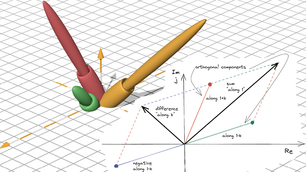
Bicomplex numbers, similarly to quaternions, have a long history, as described in the account provided by Cerroni [3], and found applications in several signal processing applications. While they have a commutative product, they do not form a division algebra, i.e. there exist non-zero bicomplex numbers whose product is zero. These numbers are multiple of
that have the following properties:

and allow the decomposition of bicomplex numbers in terms of orthogonal components.
When applied to representation in Equation 3, this orthogonal decomposition formula allows one to express ubbb(t) in terms of xbb(t) and ybb(t), which are its sideband components:

This formula is general and allows the passage from sideband components to the joint bicomplex signal representation.
Several properties characterize bicomplex numbers including a polar representation with two phases, with respect to i and j, respectively, and a modulus belonging to the set of positive hyperbolic numbers. A hyperbolic number has the form a + kb, where a and b are real components. The hyperbolic modulus (also called k-modulus) of a bicomplex number, z = a + ib + jc + kd, is defined as:

where z* = a – ib – jc + kd is the conjugate of z. z1 and z2 are the orthogonal components of z.
In the recent paper from the author[1], the properties of bicomplex numbers are used to derive effective acquisition and tracking algorithms. Their polar form, in particular, is used to derive PLL and SPLL discriminators.
Signal Recovery
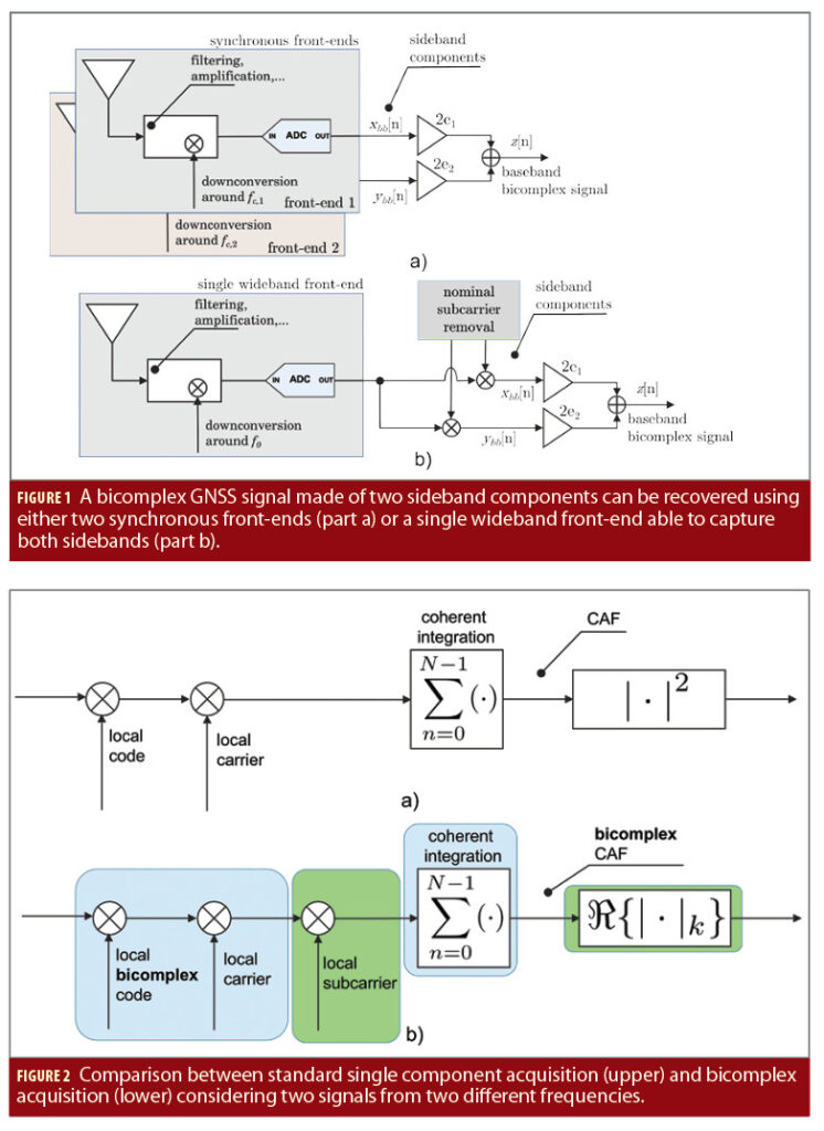
Orthogonal decomposition formula (Equation 8) allows one to recover a bicomplex baseband GNSS signal made of two components using standard receiver front-ends. Figure 1 provides two options for bicomplex signal recovery: in the upper part of the figure, two synchronous front-ends are used. The two devices are driven by the same clocks and the same sampling frequency is assumed. Each front-end provides a baseband digital representation of one sideband component. In this way, the two digital sequences, xbb[n] and ybb[n], are recovered. They are the digital sampled versions of xbb(t) and ybb(t).
In the following, n denotes the time index of a digital signal sampled at the sampling frequency, fs. Equation 8 is then used to form the corresponding bicomplex signal, denoted in the following as z[n].
A single wideband front-end also can be used. This option is illustrated in the bottom of Figure 1. In this case, the front-end captures both sidebands and downconverts the centre frequency, f0 to baseband. The baseband digital signal obtained has two sidebands approximately centered around fsub and -fsub (the Doppler effect has to be taken into account). The two baseband components are recovered by removing the nominal subcarrier: the signal is split on two branches used to isolate the upper and lower sideband components through the multiplication by complex exponentials. These are standard complex exponentials expressed with respect to the j unit and centered around fsub and -fsub, respectively. Additional filtering and decimation stages can be introduced to reduce the sampling frequency. After recovering xbb[n] and ybb[n], the bicomplex signal, z[n] finally can be formed.
Baseband Processing
After recovering z[n], baseband processing can be performed. Acquisition and tracking algorithms can be derived using the ML approach. The received bicomplex GNSS signal can be modeled as:

where ˜c(nTs-τ) is an equivalent signal code delayed by τ, the delay introduced by the communication channel. The author paper [1] provides the details on how ˜c(nTs-τ) is constructed from the codes of the sideband components. It includes amplitude factors that take into account the received signal power and the relative amplitude difference between sideband components.
The equivalent code, which is bicomplex, is multiplied by two complex exponentials modelling the effect of the carrier and the subcarrier components. These exponentials are functions of the residual Doppler frequencies, fd and fd,sub, and of the carrier and subcarrier phases, φ and φsub. In Equation 10, Ts is the sampling interval equal to the inverse of the sampling frequency, fs. Equation 10 has a functional form similar to that adopted in standard GNSS signal processing where the main differences are given by the use of bicomplex numbers and the presence of a subcarrier term. In this way, it is possible to consider two sideband components at the same time.
Equation 10 includes a bicomplex noise term, η[n], with four independent identically distributed (i.i.d.) components. The probability distribution of this noise term is used to derive the joint likelihood of N samples of z[n], which leads to bicomplex acquisition and tracking algorithms.
In particular, it is possible to show that the signal parameters, i.e. the code delay, the Doppler frequencies and the carrier and subcarrier phases, can be estimated by maximizing:
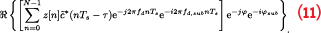
The term between square brackets defines a generalized Cross-Ambiguity Function (CAF). The maximization of Equation 11 can be performed as in standard GNSS signals processing. The CAF is expressed in polar form with two phases and a hyperbolic modulus. Code delay and Doppler frequencies are found by maximizing the real part of the hyperbolic modulus of the CAF whereas the estimates of φ and φsub are obtained as the phases, with respect to j and i, of the bicomplex CAF.
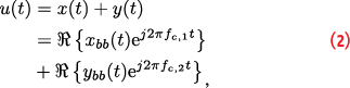
This maximization process is performed in two steps: acquisition and tracking. Figure 2 provides a comparison of a standard acquisition block, processing a single-frequency signal, and the bicomplex acquisition for the processing of a GNSS meta-signal. A similar structure is found.
In bicomplex acquisition, code delays, carrier and subcarrier Doppler frequencies are searched on a finite 3D grid. For each code delay, carrier and subcarrier Doppler frequency the CAF, defined by the quantity in square brackets in Equation 11, is computed. The summation in Equation 11 defines the coherent integration process and N, the number of samples considered, the coherent integration time. Then, the real part of the k-modulus of the CAF is computed. This defines the cost function that is maximized during the acquisition process.
Note the three-dimensional search performed during bicomplex acquisition can be reduced to a 2D search by constraining the carrier and subcarrier Doppler frequencies. Indeed, the two frequencies are related through their nominal centre frequencies. In this respect, one may search only for the carrier Doppler frequency, fd , and set the subcarrier Doppler equal to fd,sub = fd • fsub/f0.
Orthogonal decomposition formula (Equation 8) can be applied to the bicomplex CAF to express the acquisition process in terms of sideband correlators. Bicomplex acquisition can be shown to be a form of linear detector combining the CAFs of the sideband components. This type of detector was studied back in the 1950s and 1960s in the context of radar detection [4].
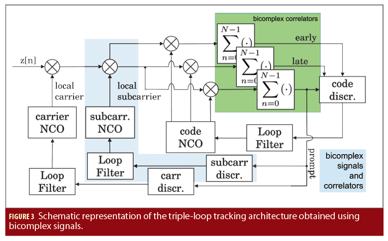
The maximization process is completed using a tracking architecture with three loops. This architecture is shown in Figure 3. It has a form similar to that of standard tracking loops where an SPLL is added to track the subcarrier component.
This tracking architecture, with standard complex signals and correlators, was suggested by the author [5] and extended to the Beidou B1C/B1I case by [2]. Bicomplex numbers provide a compact and general representation of signals and correlators with components from different frequencies. This has led to the tracking architecture shown in Figure 2. The Early, Prompt and Late correlators, found also in standard tracking algorithms, are made of four components and convey the carrier and subcarrier information. The carrier and subcarrier discriminators are easily found using the properties of bicomplex numbers and can be adapted to the cases of data and pilot signals.
Experimental Setup
The theoretical findings discussed have been demonstrated considering the AltBOC modulation adopted by the Galileo E5 signal. The AltBOC modulation is made of two components from the E5a and E5b frequencies. In this case, a single wideband front-end has been adopted and used according to the configuration illustrated in the bottom of Figure 1. For the data collection, the sampling frequency was equal to 50 MHz. The centre frequency was set to 1191.795 MHz, the centre of the E5 band. In this way, the collected sideband components were placed symmetrically with respect to the nominal subcarrier frequency at ±15.345 MHz.
The data collected was processed using a custom Python software receiver implementing the acquisition and tracking algorithms described earlier. Pilot processing was implemented; because the E5a and E5b components are transmitted with the same power and only pilot signals are considered, the local equivalent bicomplex code assumes a simple form. In particular, the equivalent code is obtained using the orthogonal decomposition formula and the E5a and E5b pilot codes as orthogonal components.
Sample Results
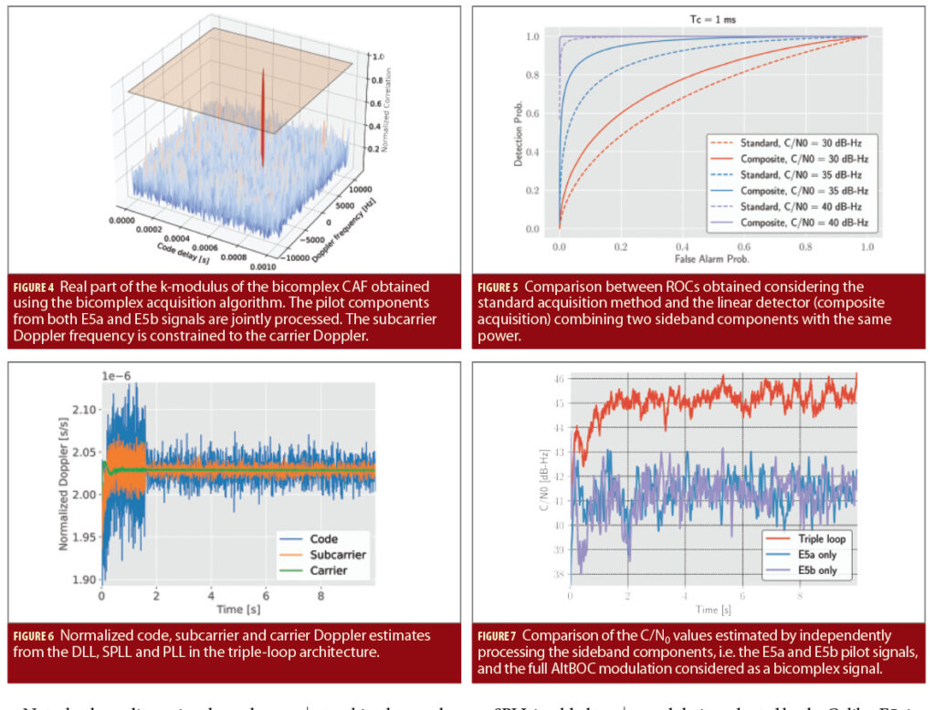
Sample results obtained through the bicomplex processing of the AltBOC signal are briefly discussed in this section. Figure 4 shows an example of bicomplex CAF obtained using the bicomplex acquisition algorithm. Only the real part of the k-modulus of the CAF is shown: this is the cost function maximized during the acquisition process. A 2D search space is considered because the subcarrier Doppler frequency has been constrained to that of the carrier component. A 1 ms integration time was selected. A clear peak emerges from the search space, revealing the signal presence. Note that the detection threshold, represented in Figure 4 as a transparent plane, has been fixed considering the false alarm probability provided by [4] for the linear detector with a number of integrations equal to 2.
To better understand the benefits of this type of combining technique, most of all with respect to the single sideband case, Receiver Operating Characteristic (ROC) curves obtained for three values of Carrier-to-Noise Power Spectral Density Ratio (C/N0) and a coherent integration time equal to 1 ms are provided in Figure 5.
For a given detector, a ROC shows the associated probability of detection as a function of the false alarm rate. A detector has better performance than another when it has a higher probability of detection for a given false alarm probability. Figure 5 shows that the combining strategy obtained using the bicomplex acquisition process always leads to better performance with respect to standard processing implemented using a single sideband component. ROC curves obtained using bicomplex acquisition are always above the corresponding curve obtained using standard sideband processing. This is expected because power from both sideband components is effectively combined.
Sample tracking results are provided in Figure 6, which shows the normalized outputs of the filters of the three tracking loops implemented. In particular, the code, subcarrier and carrier Doppler estimates are provided after normalization by the corresponding nominal frequencies.
The code Doppler frequency is normalized by fcode = 10.23 MHz, the subcarrier Doppler frequency by fsub = 15.345 MHz and the carrier component by f0 = 1191.795 MHz. After normalization, the three components overlap showing the proper functioning of the loops and the possibility of aiding, for example, from the carrier to the other components. As expected, after normalization, the carrier Doppler is the least noisy followed by the subcarrier and code components.
From Figure 6, the different processing modes implemented in the Python software receiver can be distinguished. During the first 1.7 seconds of the test, the tracking loops operate using a 1 ms coherent integration time. After this period, the software recovers the secondary codes of both E5a and E5b pilot signals and coherent integration time is extended to 5 ms. In this respect, less noisy Doppler estimates are obtained after secondary code synchronization.
Finally, Figure 7 provides a comparison of the C/N0 values estimated using bicomplex tracking and independent pilot processing on the two sideband components, the E5a and E5b signals. Sideband components have been processed independently using a standard loop architecture. A gain of about 3 dB is found when considering full AltBOC processing. This is expected because the subcarrier loop is able to coherently align the two sideband components leading to less noisy combined correlator outputs.
Conclusions
Bicomplex numbers are effective in representing, as a single quantity, GNSS signals from two different frequencies. Their polar form allows one to represent a GNSS signal as the product of three components: the code, the carrier and the subcarrier. This suggests a triple-loop receiver architecture for the wideband processing of GNSS meta-signals.
Bicomplex numbers also admit an orthogonal decomposition that allows the recovery of the original signals forming the sideband components of the GNSS meta-signal. ML estimation on bicomplex numbers has been used to derive acquisition and tracking algorithms that have been demonstrated using real Galileo AltBOC signals. The results discussed are encouraging and advocate for additional analysis to unveil the full potential of bicomplex numbers for dual-frequency GNSS signal processing.
Manufacturers
The wideband front-end adopted for the AltBOC data collection is a Universal Software Radio Peripheral (USRP)-2944R from National Instruments.
References
(1) Borio D. (2022), “Hypercomplex Representation and Processing of GNSS Signals”, Proc. of the ION International Technical Meeting of the Satellite Division of The Institute of Navigation (ION GNSS+), Denver, CO.
(2) Gao Y., Yao Z., and Lu M. (2020), “High-precision Unambiguous Tracking technique for BDS B1 Wideband Composite Signal”, NAVIGATION, Vol. 67, Issue 3, pp. 633–650.
(3) Cerroni C. (2017), “From the theory of “congeneric surd equations” to “Segre’s bicomplex numbers”, Historia Mathematica, Vol. 44, Issue 3, pp. 232-251.
(4) Marcum, J. (1960) “A statistical theory of target detection by pulsed radar”, IRE Transactions on Information Theory, Vol. 6, Issue 2, pp. 59–267.
(5) Borio D. (2014) “Double phase estimator: new unambiguous binary offset carrier tracking algorithm”, IET Radar, Sonar & Navigation, Vol. 8, Issue 7, pp. 729–741.
Author
Daniele Borio received his MS degree in communications engineering from Politecnico di Torino, Italy, and an MS degree in electronics engineering from ENSERG/INPG de Grenoble, France, in 2004. He received a doctoral degree in electrical engineering from Politecnico di Torino in April 2008. From January 2008 to September 2010, he was a senior research associate in the PLAN group of the University of Calgary, Canada. Since October 2010, he has been with the European Commission Joint Research Centre (JRC). He is currently a scientific technical officer in the JRC Food Security Unit where he is supporting the European Common Agricultural Policy (CAP) through the European satellite programs, Galileo and Copernicus.


