
A new methodology targets sub-meter GNSS accuracies in the consumer realm for applications such as augmented reality and visually impaired navigation. Recent Android RTK smartphone services in a real-time environment achieve accuracies below 50 cm. Can these be matched with PPP?
By Joshua Critchley-Marrows, Marco Fortunato and William Roberts, Nottingham Scientific Limited
Mass-market GNSS receivers are subject to intermittent and limited observation data from satellite constellations and signals. For example, in an Android smartphone, the GNSS receiver can provide at most L1/E1 and L5/E5a signals from the Global Positioning System (GPS) and Galileo constellations. Beidou and GLONASS are additionally restricted to single-frequency L1 observables.
However, given the restricted number of channels within the receiver, reception environment, internal electronic interferences and the ongoing upgrades to satellite infrastructure, multi-frequency access is limited to only certain satellites. This presents the receiver with only a select number of satellites with dual-frequency measurements, and with the remaining satellites only containing single-frequency signals. Popular GNSS algorithms such as Precise Point Positioning (PPP), using ionospheric free or ionospheric real-time models, must be adaptable to make the best use of these unfavorable conditions.
Mass market devices further present a difficult environment to the GNSS receiver in terms of signal reception. In a smartphone, the antenna is typically shared by other communication hardware, such as Bluetooth and Wi-Fi receivers. The smartphone antenna is designed for these systems, which exhibit a linear polarized signal, unlike the circular polarized form of GNSS, as well as different signal frequencies. The neighboring electronics to the receiver and antenna emit noisy electromagnetic radiation, further deteriorating the signals and increasing the signal-to-noise ratio.
These factors restrict the capability of the smartphone from a higher base performance. Smartphones and other consumer devices can realistically achieve only a few meters of accuracy in ideal conditions. This implies an open-sky, static scenario with permitted time for convergence of the positioning algorithms.
As a requirement for many new and improved location-based apps, an accuracy of 50 cm represents a reasonable benchmark to set for smartphone performances.
The methodology has been developed as part of the FLAMINGO initiative, which permits for real-time PPP and RTK GNSS positioning to be performed on a smartphone. The FLAMINGO service has achieved sub-meter positioning accuracies (below the 50 cm benchmark) in real-time. However, this high accuracy service is RTK-based and is reliant on base station infrastructure within approximately 30 km of the user.
This article explores the application of PPP as a real-time positioning service. Alternative approaches are suggested to help achieve the 50 cm benchmark. These algorithms permit for a more seamless service for the user and less cost on infrastructure.
The alternative approach modifies the traditional approach to PPP processing. It involves the pre-processing and observation state construction steps of the algorithm. Real-time PPP processing typically uses the ionosphere-free combination when dual/multi-frequency measurements are available. Removing the ionospheric term improves positioning performance. Otherwise, the single-frequency general GNSS observable model would need to be used, which can make use of the real-time ionospheric models such as Klobuchar or the State Space Representation (SSR) Vertical Total Electron Content (VTEC) product. The ionospheric term may also be estimated. Due to the intermittent nature of these GNSS signal observables, we propose a combination of these two models.
At the pre-processing stage, a filter removes poor GNSS observables. Mass market receivers in many operational environments are subject regularly to cycle slips and multipath phenomena. This filter uses both single- and dual-frequency observables, including the pseudorange, carrier phase and doppler measurements.
The signal-to-noise ratio (SNR) provides a strong indication of the measurement quality, which is especially important to the noisy environment of the smartphone. This filtration method, which has shown strong results in previous research, is combined with the more traditional satellite elevation weighting used in the Kalman filter weighting matrix.
This methodology is discussed using real-time receiver trials. A comparison is also made to a more idealized scenario, so high-accuracy performance can be demonstrated. The test environments reflect the expected scenarios of mass market GNSS users, representative of the augmented reality and visually impaired navigation cases.
Use of each technique is based on accuracy targets for certain applications. For instance, one technique may improve the vertical component. Unless however a converged solution is reached, a decrease in the horizontal accuracy might be realized.
Model Methodology
The model includes several key modifications to traditional GNSS processing:
• preprocessing stage,
• combination of both single-frequency PPP with dual-frequency ionospheric free combination of PPP and
• noise weighting by SNR and elevation. The techniques are specific to the case of Android smartphone, which differs significantly to traditional GNSS receivers.
The methodology may also be applied to IoT devices fitted with a mass-market GNSS receiver. Parameters must be calibrated according to thresholds suitable to the receiver performance.

Poor-Measurement Rejection
Smartphone measurements are highly noisy. Due to the large amount of electronics compacted inside a smartphone unit, as well as the GNSS antenna being shared with other radio frequency (RF) receivers such as Bluetooth and Wi-Fi, the environment and processing is highly unsuitable for high-accuracy positioning. In addition, due to constraints on smartphone battery and channel availability, the tracking of certain satellites and constellations is prioritized over others. This causes certain satellites or constellations to experience poorer measurements over others.
This method implements three detections strategies to remove poor measurements before being processed inside the Kalman filter. The proposed techniques are well-known to GNSS engineers but are especially important for dealing with smartphone raw GNSS measurements. The strategies are:
• Code-Minus-Carrier,
• Phase Range Rate and
• Pseudorange Rate.
If the observations do not pass all three checks, the satellite is removed. Each filter stage is important, as poor satellites are not indicated by one check alone.
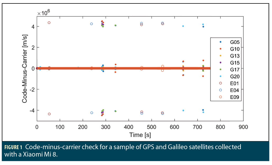
Code-Minus-Carrier. This technique considers two separate epochs of the code and carrier measurements. This is to account for the atypical carrier-phase observable that is reported through the Android Raw GNSS Measurements API. Instead of reporting a phase value aligned to the pseudorange, the accumulated delta range is prompted back to the user. The accumulated delta range is typical for smartphone handsets, also being transmitted across telecommunication networks through the Location Positioning Protocol.
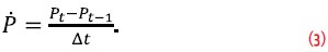
As the ADR is unaligned to the pseudorange, the code-minus-carrier check is taken over two epochs. The calculation is expressed by,
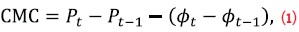
where P is the pseudorange, ϕ is the carrier phase, and subscripts t and t-1 refer to the current and previous epoch.
Over time, typically the change in pseudorange closely follows the carrier phase, as these components are highly correlated. If one observable is affected by higher noise, it is highlighted by this check. Such sources may include multipath (which can be different for each) or cycle slips (which usually only affect the carrier phase measurement).
Figure 1 gives an example of the code-minus-carrier for a sample of GNSS data collected with the Xiaomi Mi 8. Interestingly, the code-minus-carrier picks up both single-satellite anomalies in the carrier phase, but also errors for entire constellations. This may be caused by an error in the tracking solution for GPS or Galileo satellites inside the Broadcom receiver, due to constellation and satellite prioritization. This constellation should be rejected.
However, both GNSS observables may be affected at one time, so single observable checks are necessary. This may be due to high environmental noise, for example, or being able to differentiate between multipath or a cycle slip.
Phase Range Rate. The second check is to quantify the continuity of the carrier phase. The expected carrier phase should follow the reported doppler shift. A deviation from this check may indicate an error in the receiver clock, or a cycle slip.
The difference between the current and the expected phases may be found by
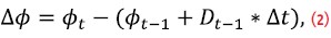
where D is the Doppler shift in the phase and Δt is the time interval between the current and previous epoch.
The phase range rate check is illustrated in Figure 2. The importance of the previous check is also shown, as all constellation anomalies may not be picked by this check alone. However, errors to the carrier phase alone may be picked up by this check only. Figure 1 and Figure 2 are very similar, but the value threshold differs between the two methods. It is important both checks are employed.
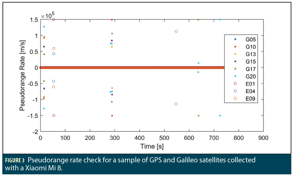
Pseudorange Rate. The pseudorange rate should fall within a set of predefined values. The limits are set by the extremities of satellite and receiver dynamics, as well as clock drifts. A pseudorange rate outside a predefined value, largely associated to the type of receiver, can highlight a corrupt measurement.
The pseudorange rate may be calculated by the simple operation
Any anomaly to the pre-defined thresholds of the pseudorange rate would be removed.
The pseudorange rate performed on the same set of data is presented in Figure 3. This check picks up erroneous observables to the pseudorange. In Figures 1 and 2, errors to a single Galileo are highlighted. Figure 3 emphasizes errors to all three Galileo satellites.
SFDF Combination
In GNSS modelling, each error term should be accounted for to reduce the error, such as the satellite clock and ephemeris, troposphere and code and phase biases. If the receiver has two or more frequencies, signal combinations may be applied to remove error terms.
The ionospheric-free combination may remove the ionospheric term from the observables. Alternative methods to account for the ionosphere include the Klobuchar and NeQuick models, which form part of the GPS and Galileo navigation messages respectively. If used in a post-processing case, the Ionospheric Map Exchange file may be used, calculated by various GNSS analysis centers such as the Jet Propulsion Laboratory or Centre National D’Etudes Spatiales.
The PPP technique may then also use precise satellite ephemeris, clocks and code biases to account for unknowns in the geometric range term and satellite clock. This data may be retrieved from accurate post-processed precise products or real-time RTCM SSR messages.
Code biases are also available through precise products from analysis centers, or as an RTCM SSR stream.
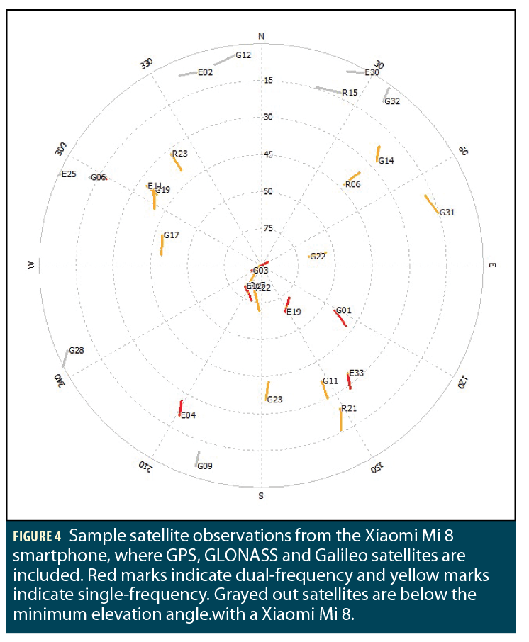
The SFDF is proposed to compensate for the mix of L1 and L1/L5 satellite observations from an Android smartphone, or in other mixes of multifrequency observations from mass-market receivers. Figure 4 gives an example of observed satellite and their available signals. Only a limited number of satellites include dual-frequency observations; the rest are single-frequency. The number of observations is highly restrictive if considering dual frequency alone.
The pairing of these techniques may be incorporated into a Kalman filter algorithm like the traditional approaches of single-frequency or ionospheric free combination. The changes are only simple modifications to the state and innovation vectors.
The pseudorange P and carrier phase ϕ may be written as vectors for single-frequency observations of a satellite and the linear ionospheric free combination of dual-frequency,
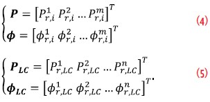
Where subscript r refers to the receiver number, subscript i refers to the frequency number, subscript LC refers to the ionospheric-free linear combination, and m and n are the number of single and dual-frequency observations respectively. The vectors are part of the innovation vector of the Kalman filter,
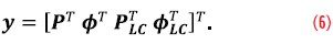
The algorithm is designed to work for the real-time scenario, relying on SSR corrections to solve for various unknowns. From the current release of RTCM 3.3, only the precise orbits, clocks and code biases are known. The ionosphere, troposphere and phase biases will be a part of future releases. As the ionosphere and troposphere may be calculated by pre-existing models, the Klobuchar and Saastamonien respectively, these terms may also be removed. The phase bias is incorporated into the unknown phase bias term and is solved in the state vector.
The state vector is formed by,
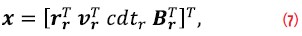
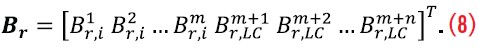
where rr is the receiver coordinates in the Earth-Centered, Earth-Fixed (ECEF) reference frame, vr is the receiver velocity, cdtr is the receiver clock and Br is the phase bias vector,
For a static case, the velocity term may be set to zero.
The Extended Kalman filter equations may then be formed and applied based on these state and innovation step definitions.
Model Weighting
Traditional GNSS uses an Extended Kalman filter weight based on the satellite elevation. This is a reasonable assumption, as the level of noise the signal encounters increases extensively at low elevations, such as built landscape and atmospheric path distance. An additional parameter to consider is the signal-to-noise ratio. Use of a weighting dependent on the signal-to-noise ratio has also been in practice for several decades.
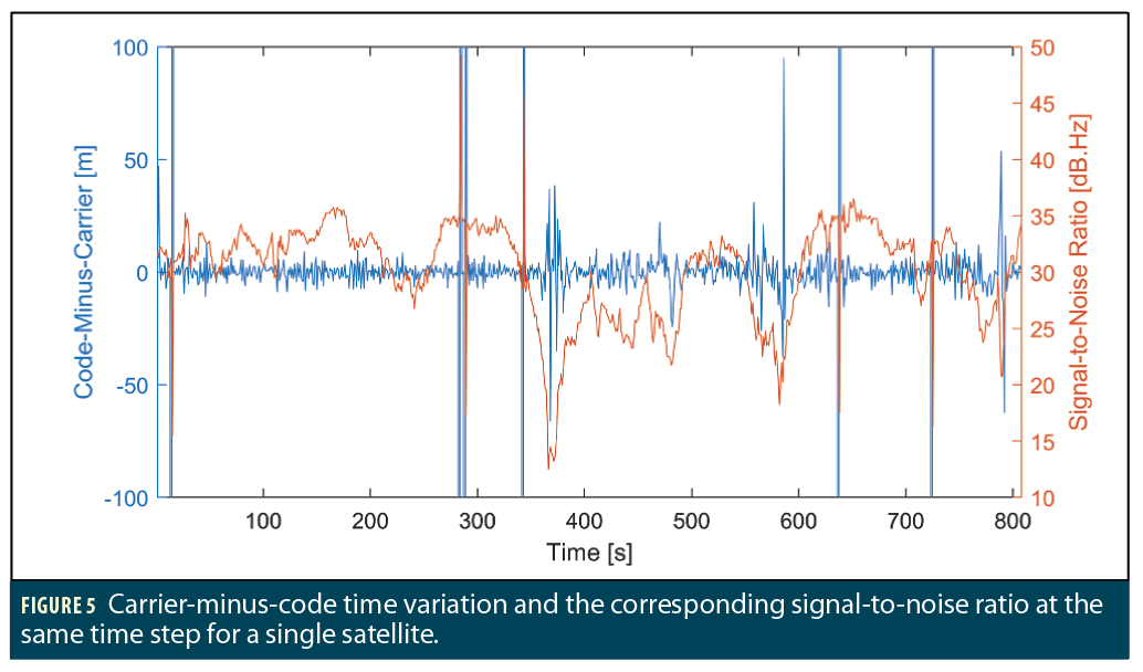
The importance of the signal-to-noise ratio is addressed in Figure 5. As discussed previously, the code-minus-carrier phase is an indicator of the noise of the measurement. By overlaying this with the SNR, as in Figure 5, a correlation is evident between the two variables.
Considering the shared and undesirable nature of the antenna for GNSS, all possible parameters which may reflect the measurement quality of the antenna should be accounted for. As the elevation is still an important parameter for the measurement noise weighting, especially for a single-frequency receiver, combining both terms as a weight is written as
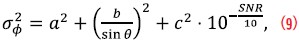
where a is the base term of carrier phase error standard deviation, b is the elevation dependent term of carrier phase error standard deviation, θ is the elevation angle of the satellite, c is the signal-to-noise ratio dependent term of carrier-phase error standard deviation and SNR is the signal-to-noise ratio.
Implementation and Test Results
Apps have been specially made by NSL that use GNSS data in an RTCM format to perform both PPP and RTK processing. Only PPP is considered in this article.
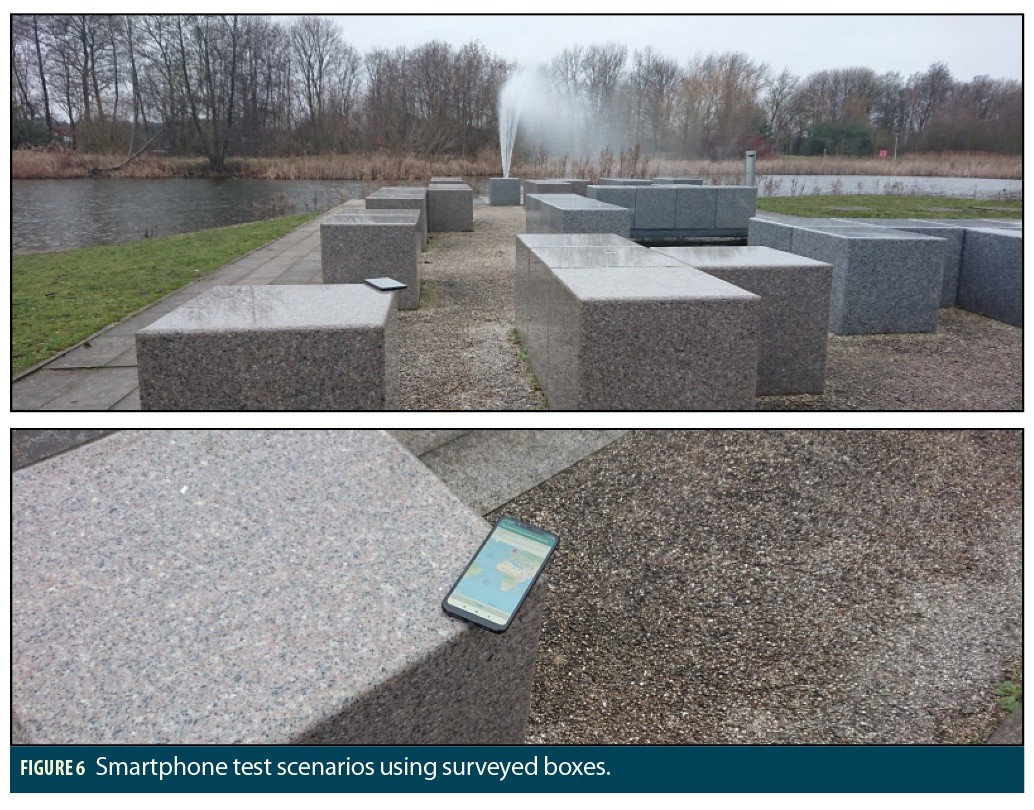
As a point of comparison, analysis is also conducted in a post-processing case. Post-processing is considered to establish the key differences from real-time. Test data is collected at a special smartphone test arena established at the NSL premises (Figure 6).
This contrasts with other test scenarios within the literature, where the smartphone may be placed in an isolated chamber, or on a metallic choke ring, in an attempt to improve performances. There is no special equipment used for these tests. The real-time application is opened, and processing begins at once.
Post-Processing Ideal Case
The ideal case considers a data sample collected from the test scenario illustrated in Figure 6. The data is post-processed, implementing approaches that are not possible in a real-time scenario. For this test, the GNSS observable data is collected using the NSL RINEX logger app, rinex ON.
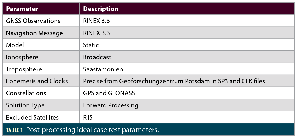
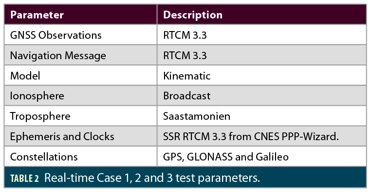
The test parameters are summarized in Table 1. Specifically, post-processing enabled:
• Removal of the Galileo constellation, as the satellite effects appeared to deteriorate the solution.
• Excluding GLONASS satellite R15, as it also seemed to deteriorate the results.
• Using precise ephemeris and clock files Geoforschungzentrum Potsdam.
• Setting solution to a static case, which fixes the velocity state parameter to zero.
Each of the improvements would not be possible nor suitable in a real-time scenario. However, these modifications improve the scenario’s performance.
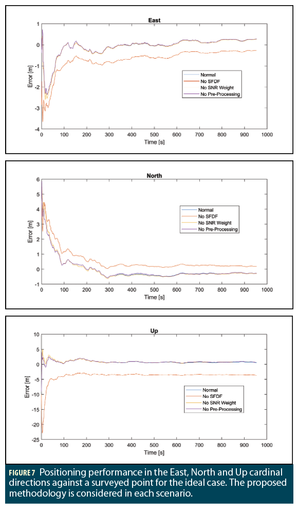
Figure 7 presents results for the ideal case, in North, East and Up direction. The methodology is implemented. To study the influence of each step, a single technique is removed with each line. No SNR weighting denotes the model weighting technique of Equation (9).
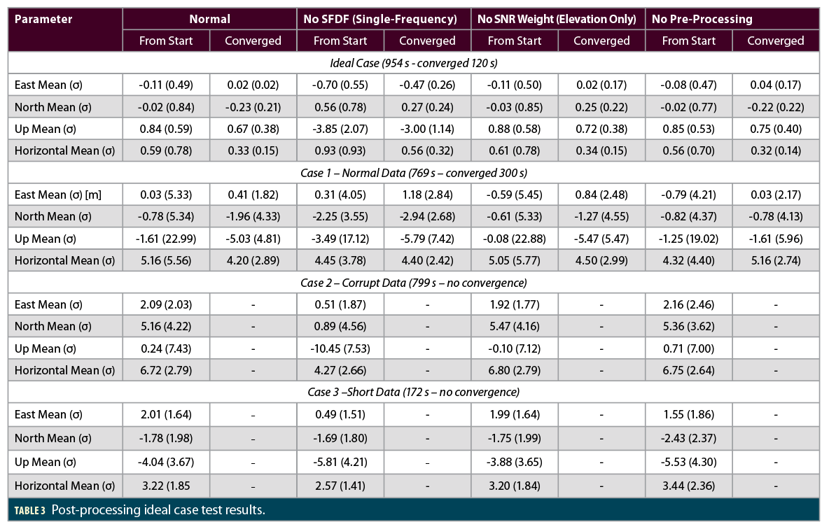
Table 3 presents the results of the post-processed case. The solution converges to a final position, with a convergence time of approximately 120 s. This fast convergence is caused by having a fixed static position, reducing the number of state variables.
The results of this ideal case are a highly accurate solution. After convergence, the solution realizes an accuracy of 0.33 m in the horizontal and 0.67 m in the vertical. Further improvements may be made by using additional precise products, smoothing of the pseudorange and input of an accurate solution guess.
A difference is seen in using the SFDF model. By removing the ionospheric term in a dual-frequency combination, which generally affects the vertical direction more than the horizontal, there is a distinct improvement made in the Up component of the final solution. This has an indirect effect in the East and North, where the converged solution improves.
The effect of the SNR weight is minor, since the solution is static, and noise has already been partially filtered. However, there is a small improvement to the solution precision with the introduction of a combined SNR- and elevation-based measurement noise model.
A pre-processing filter contribution is negligible, as the real-time filtration has been largely replaced by making a post-processed modification to the model.
Real-Time Cases
Like the post-processed case, the real-time solution is realized in a static case, as illustrated in Figure 6. The data is processed in a real-time environment, using a specially configured mobile app designed and developed by NSL, where all processing is run through the app..
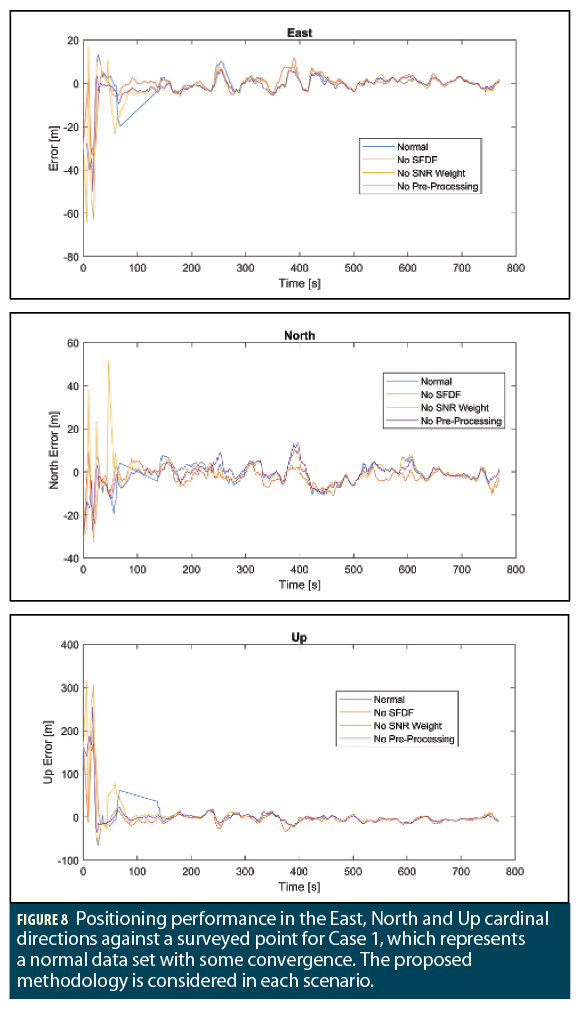
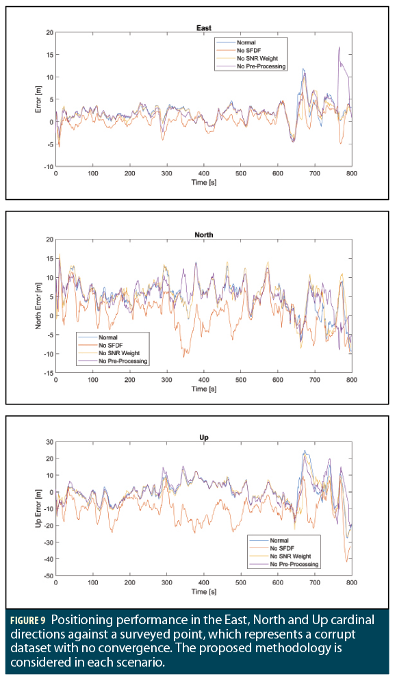
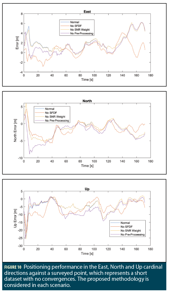
Three cases are realized for the smartphone, each effected by the smartphone’s difficult operational environment. The first case is a normal dataset, with no anomalies present in the data. In the second case, there was a failure in use of SSR corrections for the Galileo satellite, as well as jumps to both the carrier phase and pseudorange observation, occurring approximately once every minute. Each of these jumps only effected a single constellation at a time, so these observations could be removed by the pre-processor. The third case is a very short dataset, representative of the smartphone user running an application for only a few minutes.
The parameters of each test case are the same. These parameters are presented in Table 2. In Figures 8 to 10, the results of each case are presented. The solutions of the tests, in terms of the mean and standard deviation, are presented in Table 3.
The results of the final solution are much less accurate than the ideal case, where each case does not converge fully. A partial convergence is seen in case 1, which is taken at the 300 s mark. The precision of the final solution is improved after this point. Prior to this, some solutions fail to identify a reasonable value, hence gaps in the data. The maximum value of the innovation step in the Kalman filter is set to 30 m.
A key difference to note from the ideal case is using final solution for orbit and clock parameters of the satellites. The use of much more accurate parameters for the PPP model improves greatly the ability to converge to more accurate solutions.
The accuracy improvement of the SFDF model is clear after convergence. The mean improves, however an improvement to precision is not clear in the horizontal. The precision in the up component is representative of the improved vertical accuracy. Prior to convergence however, the benefit of SFDF improvement is not evident except for the vertical component alone.
This highlights the importance of using SFDF for certain applications. If developing an augmented reality application, the vertical component is very important. However, if a fitness app is developed, where performance of a runner in terms of position and speed is desired, it may be more important to focus on the horizontal accuracy only, and so the effects of the SFDF technique are undesired.
The SNR weight improves the precision for East, North and Up components. However, this is also not evident unless the solution converges, and so is only evident in Case 1. At the start of data collection, the satellite receiver requires time to lock and track certain satellites. The SNR may not be directly correlated with the observable noise during this period, and only after a period may the SNR weighting be used.
Scenarios requiring a high precision might use the SNR weight, and so for a surveying application, the user is content to wait for a period to achieve a position fix with a high precision. However, for a navigation app, the user is impatient and so an accurate solution average is all that is important.
The benefits of pre-processing are not evident from the results. In terms of solution accuracy and precision, losing satellite observables reduces the performance achieved. However, for applications that require high solution integrity, rejecting very poor observations might be more desirable. Such solutions were illustrated in the post-processed scenarios of Figures 1 to 3.
Conclusion
The methodology for real-time GNSS positioning in mass-market receivers is designed to deal with intermittent GNSS signal observables, noisy environments and minimal signal information from the reciever.
The ideal case shows an accuracy of 0.33 m in the horizontal and 0.67 m in the vertical. The benefits of the SFDF technique, pre-processing and SNR weighting are highlighted with improved vertical accuracy and precision of the solution.
This performance is not translatable to real-time implementation. Use of the techniques in the methodology should be decided on based on the desired application. Improved vertical accuracy is demonstrated with the SFDF technique, but a correlated increased accuracy in the horizontal is not guaranteed.
Smartphones are not limited to GNSS in their positioning capabilities. In the ideal case, a static filter was imposed on the model. In a smartphone, a combined approach with use of other sensors may help in deciding if the device is static, and then imposing this criterion to the filter.
The ideal case also highlighted an improved performance with more accurate ephemeris and clock information. Real-time broadcast of SSR corrections is still an emerging field of GNSS research and development, and so there is still strong potential for the sub-meter target.
Sub-meter accurate PPP in a real-time implementation is yet to be realized. Smartphones present a difficult environment for positioning. High accuracy GNSS will, with persistence, yield great rewards.
Acknowledgment
The authors acknowledge the support of the Geodesy and Geomatics Division, Department of Industrial, Civil and Environmental Engineering, Sapienza University of Rome. FLAMINGO received funding from the European GNSS Agency under the EU’s Horizon 2020 research and innovation programme under grant agreement No 776436.
Authors
Joshua Critchley-Marrows, GNSS engineer withNottingham Scientific Ltd. (NSL), is project and technical lead of activities across UK, Europe andAustralia, including smartphone high-accuracy services, broadcast of satellite data in telecomm networks and satellite mission feasibility studies. He hasHonor degrees in Engineering (Aeronautical (Space))and Science (Advanced Mathematics) from the University of Sydney.
Marco Fortunato is a Ph.D. student in Geodesy and Geomatics Division at the Sapienza University of Rome, working also part-time at NSL. His studies are focused on improvements to achievable performances with mass-market GNSS receivers andAndroid smartphones, especially in kinematic applications.
William Roberts is operations manager at NSL, where he leads NSL’s services and solutions for GNSS space, ground and user segment planning, GNSS forland and infrastructure monitoring and high accuracySmartphone positioning. He holds a Ph.D. in satellite geodesy from the University ofNewcastle-upon-Tyne


