
The Smart Tachograph (ST), the new revision of the Digital Tachograph (DT), aims to improve safety in the transportation sector by monitoring the behavior of commercial drivers. For this purpose, data from several sensors, including a GNSS receiver, are recorded, processed and cross-validated. In this article, the motion conflict procedure adopted by the ST is reviewed and experimentally evaluated using data collected in light urban and highway environments.
Violations of road rules such as prolonged driving periods and infringements to speed limits can entail severe safety risks. For this reason, the adoption of the Smart Tachograph (ST), the new revision of the Digital Tachograph (DT), has been mandated in the European Union (EU). The ST is an electronic device that aims to improve safety in the transportation sector by monitoring driver behavior. Starting in June 2019, its installation will be mandatory in new commercial vehicles with a mass of more than 3.5 tonnes (3.5 metric tons) in goods transport and carrying more than nine people, including the driver, in passenger transport. The ST records information about driver behavior such as driving time, rest periods and breaks: by monitoring driver behavior, the ST is expected to discourage the violation of road rules and to improve road safety.
The legal framework of the ST has been recently revised according to Council Regulation (EU) No. 165/2014 listed in Additional Resources. Moreover, the technical specifications of the existing DT were discussed with stakeholders including law enforcers, manufacturers and service providers. This process led to the definition of new technical specifications of the ST that can be found in Council Regulation (EU) No. 799/2016 listed in Additional Resources.
A key feature of the ST is the adoption of an interface with Global Navigation Satellite Systems (GNSS), including the European GNSS, Galileo and EGNOS. A GNSS receiver will be used to record positions related to the daily work periods including the start and stop locations of the commercial vehicle. In addition to GNSS data, the ST will access information from other sensors such as the on-board odometer. The availability of data from different sensors allows the ST to perform periodic consistency checks to prevent the risk of data falsification. In this respect, Regulation (EU) No. 165/2016 prescribes the cross-validation between GNSS and motion sensor data to mitigate the risk above. For example, a motion conflict will be generated if a significant discrepancy between GNSS and odometry information is observed. These procedures have been implemented to reduce the risk of GNSS spoofing and data manipulation.
This article reviews the motion conflict procedure adopted by the ST and provides an experimental evaluation of the mechanism used for speed data verification. While logistic and cost reasons prevented the use of a real commercial vehicle above 3.5 tonnes, the experimental setup adopted and the measurement campaigns conducted are considered realistic. Two scenarios were considered and three different vehicles were employed for the data collections. Several hours of data were recorded and used for the experimental evaluation of the ST speed verification procedure.
The analysis shows that, with the new ST, it is not sufficient to falsify GNSS information alone and an attacker has to forge data from both the vehicle sensor and the GNSS receiver simultaneously, which makes the attack implementation quite difficult.
The Smart Tachograph
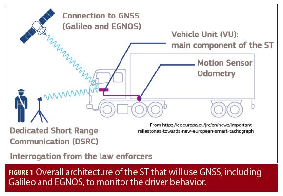
Different architectures can be adopted for the implementation of the ST (see the article by Baldini et alia, 2018, Additional Resources). In all architectures, the main element of the ST is the Vehicle Unit (VU), which is responsible for the different functions of the ST including the collection of data from different sensors and data verification. The VU is connected to the motion sensor, whose purpose is to provide motion data, which reflect the vehicle’s speed and distance travelled. The VU is connected to a GNSS receiver that provides Position, Velocity and Time (PVT) information. GNSS data are used for different operations including the motion conflict detection process described below. The ST regulation mandates the use of the European GNSS, Galileo and EGNOS, that can be used in conjunction with other GNSS. The VU records information including the different events triggered by the tests performed by the device. Law enforcers can interrogate the ST through Dedicated Short Range Communication (DSRC) link (based on CEN-DSRC standards using the 5.8 gigahertz band). Depending on the result of the interrogation, law enforcers can decide to stop the vehicle and proceed with further investigations. A schematic representation of the ST architecture is depicted in Figure 1.
Motion Conflict Detection
The ST will verify the quality of GNSS data by comparing the speed obtained from the GNSS receiver with that provided by other sensors. A possibility is to use the speed obtained from the on-board odometer. In this respect, the VU can use the speed provided by the odometer, Sodo(t), and recovered through an On-Board Diagnostics (OBD)2 interface. We adopted this approach since OBD2 data readers are widely available on the market and the vehicle speed can be easily obtained by interrogating the vehicle OBD system. This system adopts a serial protocol where information is provided as a response to a data interrogation performed by sending a Parameter IDentifier (PID). In particular, the vehicle speed is retrieved using PID 13. The odometer speed is provided in an asynchronous way and thus Sodo(t) is sampled at irregular time instants, t = tn. The vehicle speed is provided as an unsigned 8 bit integer with values in the [0, 255] km/h range. The speed is quantized with a 1 km/h resolution.
GNSS receivers usually provide 3D information and the vehicle velocity can be obtained as a 3D vector. In this work, we considered the case where the 3D velocity vector is provided by the receiver and computed from Doppler measurements. In this case, the speed is derived as the absolute value of the velocity vector:

where VE(t), VN(t), and VU(t) are the three velocity components expressed in a local East, North, Up (ENU) frame.
It is noted that the ST regulation (European Commission 2016) prescribes the usage of the National Marine Electronics Association (NMEA) 0183 protocol for the data exchange between GNSS receiver and VU. In this case, SGNSS(t) is provided directly as part of the NMEA Recommended Minimum Data (RMC) sentence. We have tested this case by including a smartphone in the data collection system and by recording RMC sentences directly providing the GNSS-derived speed. This case is detailed later in the article.
GNSS measurements are provided at regular time instants and SGNSS(t) is sampled at t = nTs where n is the time index and Ts is the sampling interval. GNSS and odometry data are not synchronized and thus a synchronization mechanism needs to be implemented. For this reason, the procedure illustrated in Figure 2 has been adopted.
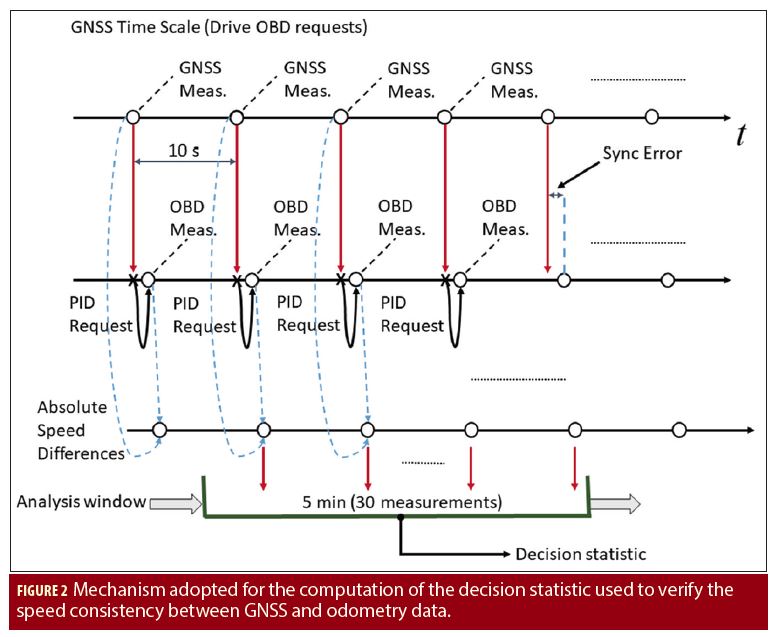
The GNSS time scale is used to generate PID requests for the OBD interface. These requests trigger the provision of new odometer measurements that can be compared with GNSS information. A small latency is introduced between the generation of the data request and the provision of Sodo(tn). This causes a small synchronization error between SGNSS(nTs) and Sodo(tn). This error is however small and the decision statistics considered by the ST regulation have been designed to be tolerant with respect to these types of errors.
The synchronization approach described in Figure 2 can be adopted for a real-time implementation of the motion conflict detection strategy prescribed by the ST regulation. In the data collections performed and described in the next sections, GNSS and OBD data were collected in an independent way. The synchronization approach described in Figure 2 was then implemented in post-processing. In particular, the data collected were roughly synchronized using a correlation approach. This synchronization was performed only once at the beginning of the dataset. The approach in Figure 2 was then implemented by associating to each GNSS measurement the next available odometer speed with the closest time stamp. Additional details on the synchronization procedure adopted in post-processing can be found in our article listed in Additional Resources (Borio, et alia 2018).
Using SGNSS(nTs) and Sodo(tn), it is finally possible to compute the speed differences that are the basic signals used for the computation of the decision statistics:
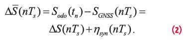
In the previous equation, the symbol – denotes the impact of synchronization errors. ΔS(nTs) is the ideal speed difference affected by the synchronisation error, ηsyn(nTs). According to the ST regulation, speed differences should be computed at least every 10 seconds. For this reason, Ts = 10 s was adopted.
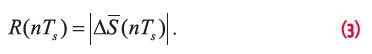
The decision statistics are finally computed using the approach described at the bottom part of Figure 2. The absolute values of the speed differences are at first computed:
An analysis window is then used to select 5 minutes of data corresponding to N = 30 measurements for Ts = 10 s. The selected measurements are then used for the computation of the decision statistics. According to regulation (EU) No. 799/2016 (European Commission, 2016), the final decision statistic should be computed as the trimmed mean of the 30 measurements selected, where 20% of the observations are discarded. When N = 30, the six absolute speed differences with the largest values are removed and the mean absolute speed difference is computed and used to determine motion conflicts. In our work, we also considered the median absolute speed difference as a comparison term. In this case, the decision statistic is the sample median of the measurements selected by the analysis window.
The decision statistics are compared with a decision threshold equal to 10 km/h. If this value is exceeded, a motion conflict event is triggered and recorded in the VU.
Experimental Setup
In order to experimentally evaluate the motion conflict detection mechanism described above, several data collections were performed considering different vehicles and scenarios. Different car models were considered since each vehicle implements slightly different OBD interfaces. Our goal was to evaluate possible inter-model differences by considering different car models. Three vehicles were used for the analysis and are denoted in the following as Model 1, Model 2 and Model 3.
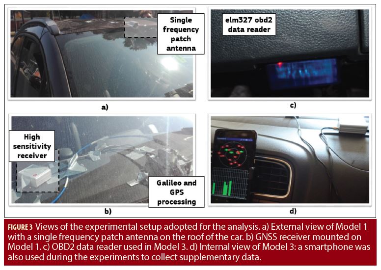
In all cases, a single frequency GNSS high sensitivity module able to provide raw GNSS observables was used. The module was configured to use both GPS and Galileo. The use of Galileo provides benefits in terms of signal availability and position accuracy. We analyzed these aspects in our recent paper listed in Additional Resources. In all cases, a single frequency patch antenna was used. Depending on the test, different antenna positions were considered. Figure 3 provides different views of the experimental setup adopted for the data collections. Figure 3 a) shows the rooftop of Model 1 with the single frequency patch antenna taped above the front windshield. In the tests performed using Model 3, the antenna was placed inside the vehicle and below the front windshield as shown in Figure 3 d). Odometry data were collected using ELM327 OBD2 data readers. The device used for Model 3 is shown Figure 3 c). GNSS and odometry data were recorded using a laptop.
In order to test the impact of the GNSS receiver and to evaluate the use of RMC NMEA sentences, a smartphone was placed inside the vehicle and used to collect supplementary data. The low-cost GPS/GLONASS smartphone used for the tests with Model 3 is shown in Figure 3 d).
The experiments considered two types of scenarios:
• Light-urban environments
• Highway experiments
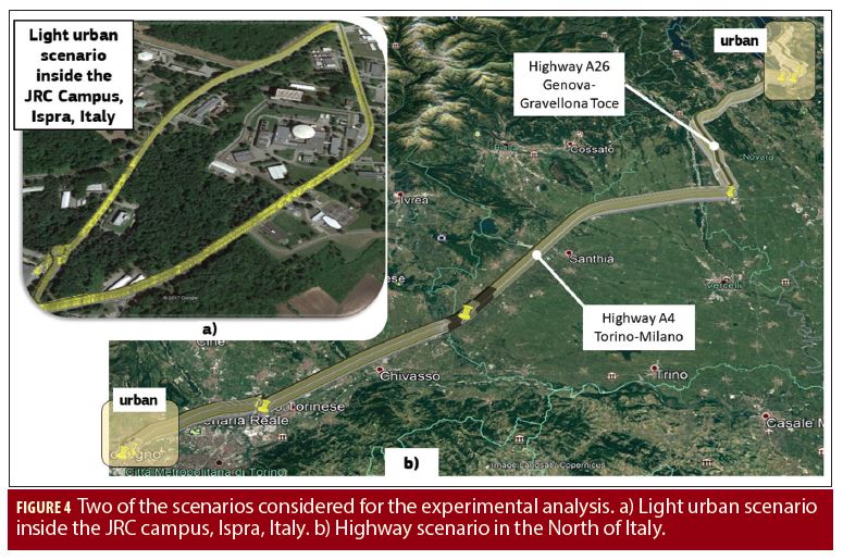
The first type of environment was analyzed by performing several tests inside the Joint Research Centre (JRC) campus in Ispra, Italy. In this case, the closed trajectory illustrated in Figure 4 a) was repeated several times over several days. Model 1 and 2 were used for the tests and a total of 8 hours of data were collected.
The highway experiments were performed using Model 3 and considered a section of about 130 kilometers of Italian highways in the Turin/Milan area. The test was repeated several times. In the following, we will detail the results obtained considering data collected in August 2018. The results are consistent with the findings described in our paper listed in Additional Resources (Borio et alia 2018).
The trajectory of this test is illustrated in Figure 4 b). It also includes two urban areas, at the beginning of the test. These urban sections can be easily identified from the speed profile recorded.
Experimental Results
The results obtained during the experimental campaigns discussed above are briefly described in the following. Specific focus is devoted to the results obtained under nominal conditions. The impact of simple data manipulations is analyzed at the end of the section.
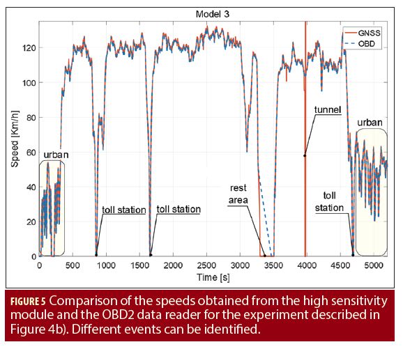
In all the experiments performed, a good agreement between GNSS and odometry data have been observed. The speeds from the GNSS receiver and the OBD2 data reader recorded for the experiment described in Figure 4 b) are compared in Figure 5. The two speed curves overlap for almost the total duration of the test. In the plot, different events can be identified such as the urban sections of the experiments, characterized by moderate and more variable speed profiles, and the stops at the toll stations. GNSS and odometry data differs only when the car passes under a tunnel of about 670 meters. In this case, the GNSS receiver stops providing valid speed values. The GNSS receiver provides a zero speed and a spike is observable after about 4,000 seconds from the start of the test.
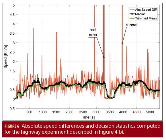
The absolute speed differences and the two decision statistics (trimmed mean and median) obtained for the test analyzed in Figure 5 are provided in Figure 6. For the total duration of the experiment, the absolute speed differences assume values below 3 km/h. Spikes above this value occur sporadically and mostly in correspondence of specific events such as the stop at a rest area or the passage under a tunnel. The two decision statistics used for motion conflict detection are based on robust operators, the trimmed mean and the median, that have been selected for their ability to reject outliers and sporadic anomalous speed difference values. For this reason, the decision statistics are only marginally influenced by the presence of speed differences above 3 km/h. The decision statistics evaluated in Figure 6 assume values around 1 km/h that are significantly below the 10 km/h threshold prescribed by the ST regulation.
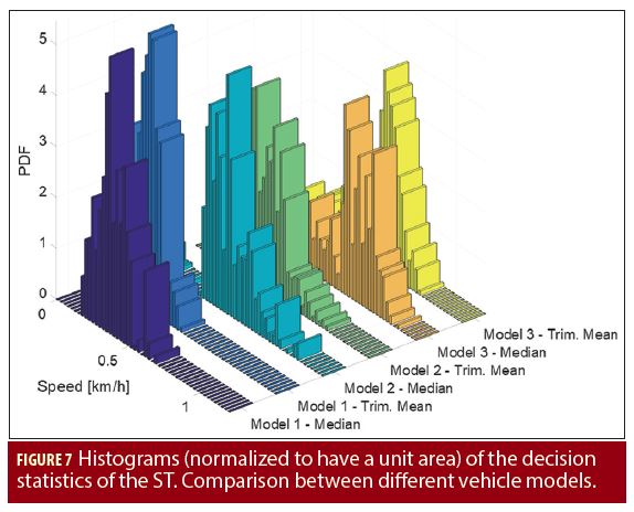
The behavior of the decision statistics is analyzed in Figure 7, which compares the histograms obtained for the decision statistics when considering the three models. The histograms related to Model 1 and 2 have been obtained using the data collected during the tests performed for the light urban scenario on the JRC campus.
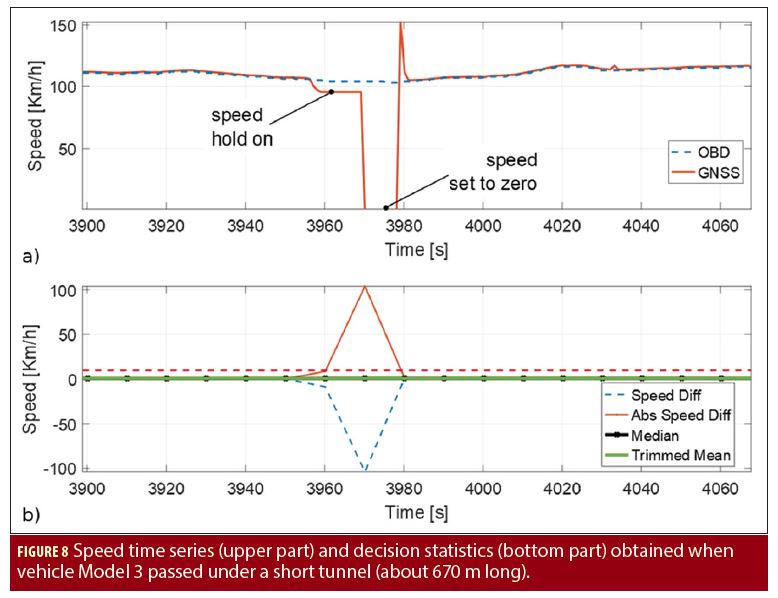
The histograms for Model 3 have been obtained using the time series shown in Figure 6. In all cases, the decision statistics assume values below 1.5 km/h. Model 1 and 2 are characterized by lower maximum values that are below 1 km/h. This could be due to the location of the antenna that was placed on the roof of the vehicles. For Model 3, the antenna was inside the vehicle. A second difference is also related to the fact that the tests performed for Model 3 include tunnels and stops that caused sporadic spikes in the absolute speed differences. Despite these differences, the decision statistics are significantly below the decision threshold and robust to different errors, including residual synchronization effects. In all cases, the two decision statistics, median and trimmed mean, assume similar values and have a similar behavior when data are collected in the absence of manipulations. The impact of tunnels on the decision statistics is analysed in Figure 8. In the absence of GNSS signals, the GNSS receiver propagates the user’s position using the last velocity information. This operation is performed for 10 seconds. If the GNSS outage is longer than 10 seconds, the receiver provides an invalid speed equal to zero. This behavior is clearly observable in the upper part of Figure 8, which shows the speed time series provided by the GNSS receiver and the odometer. Invalid GNSS speed values generate large speed differences that can affect the decision statistics. In this case, the tunnel is quite short (about 670 meters) and the number of invalid measurements is not sufficient to significantly bias the decision statistics, whose behavior is analyzed in the bottom part of Figure 8. As already mentioned, the decision metrics selected by the ST regulation are robust to data gaps. The median decision statistic can tolerate data gaps up to 150 seconds while the trimmed mean will start to be biased when the data gaps last more than 60 seconds.
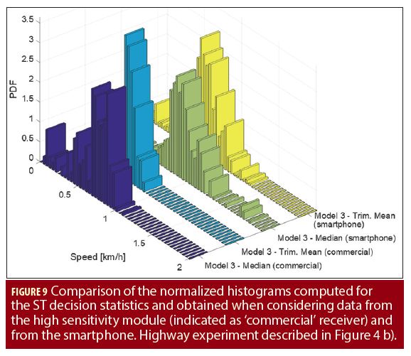
The results presented above were obtained using a high sensitivity module and a patch antenna. The case where a low-cost smartphone GNSS receiver is adopted is considered in Figure 9, which compares the histograms of the decision statistics obtained when using different GNSS receivers. The histograms have been evaluated by considering the same scenario, i.e. the highway test described in Figure 4 b). When smartphone data obtained from NMEA RMC sentences are used, larger speed differences are obtained. This is due to the lower quality of the GNSS receiver and of the antenna integrated within the smartphone. Despite the lower quality of the measurements, the decision statistics assume values significantly lower than the 10 km/h threshold prescribed by the ST regulation. From the histograms reported in Figure 9, it emerges that the decision statistics computed using the smartphone data are characterized by maximum values lower than 2 km/h.
These results show that the ST test statistics are resilient to false alarms, even when low quality devices are used. The analysis shows that the decision threshold provides sufficient margin to account for different errors, including synchronization effects. Moreover, the test procedure is resilient to data gaps on GNSS and odometry data.
In our work listed in Additional Resources, we have tested the impact of data manipulation on the ST decision statistics. We have considered the introduction of relative delays between odometry and GNSS data and the impact of data scaling. The introduction of relative delays between time series allows one to study the impact of synchronization errors, for short delays, and of meaconing attacks, for long delays. Effective decision statistics should be tolerant to small synchronization errors and be able to detect discrepancies when relatively long delays between time series are introduced.
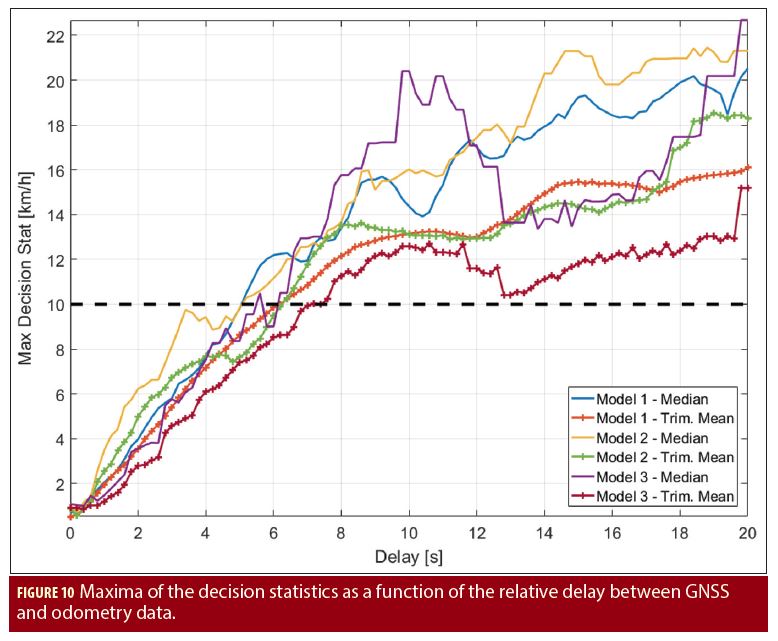
These effects are analyzed in Figure 10 that shows the maxima of the decision statistics as a function of the relative delays between GNSS and odometry data. All three vehicles are considered along with the two decision statistics. From the figure, it emerges that the detection threshold is not exceeded for relative delays lower than approximately 5 seconds. Larger delays trigger threshold crossing. The curves for Model 1 and 2 have been obtained using the data collected on the JRC campus, whereas the plots for Model 3 were obtained using the highway data. Despite these differences, consistent results were obtained.
These results show that the decision statistics selected for detecting a motion conflict can tolerate a significant latency (synchronization error) between GNSS and odometry data. The second conclusion is that a simple meaconing attack seems unlikely to be successful. The ST decision statistics are able to detect inconsistencies between motion data even when only a few seconds of delay are introduced. When GNSS and odometry data come from different and unrelated scenarios, the decision statistics reach higher values than those shown in Figure 10. For this reason, a meaconing attack can be successful only if both sensors are compromised, which can be quite difficult to achieve.
When data are manipulated by scaling one of the time series, the ST consistency mechanism allows discrepancies lower than the decision threshold. These discrepancies depend on the speed profile. For example, if an average speed of 50 km/h is adopted by the driver, a maximum 20% scaling can be applied to one of the time series. This scaling corresponds to a discrepancy of 10 km/h and is equal to the detection threshold. This is the maximum error allowed by the decision threshold. More details on the effects of this type of data manipulation can be found in the authors’ paper listed in Additional Resources.
Conclusions
This article evaluated the performance of the decision statistics introduced by the ST regulation to verify the consistency of speed data from different sensors. The speed consistency mechanism has been experimentally characterized using three vehicles and considering different scenarios.
The experimental analysis showed that the test statistics have been designed to have a low number of false alarms and to be robust to different errors such as data gaps and synchronization errors. In the experiments conducted no false alarm was recorded. The decision threshold equal to 10 km/h defined in the ST regulation provides sufficient margin against false alarms.
The test statistics are also robust to latencies between GNSS and odometry data. Moreover, the experimental analysis shows that the decision statistics are effective against data manipulation forms such as meaconing attacks and data scaling. In this latter case, only discrepancies lower than the 10 km/h threshold are undetected by the tests prescribed by the ST regulation.
Manufacturers
The GNSS high sensitivity module used for the experiments is a u-blox M8T device from u-blox, Thalwil, Switzerland.
Additional Resources
[1] Baldini, G., L. Sportiello, M. Chiaramello, and V. Mahieu, “Regulated applications for the road transportation infrastructure: The case study of the smart tachograph in the European Union”, International Journal of Critical Infrastructure Protection, Vol. 21,pp. 3-21, June 2018
[2] Borio, D., E. Cano, and G. Baldini, “Speed Consistency in the Smart Tachograph”, Sensors 18, No. 5, pp. 1-21, May 2018
[3] European Commission, “Regulation (EU) No 165/2014 of the European Parliament and of the Council of 4 February 2014 on Tachographs in Road Transport,” online, http://eur-lex.europa.eu/legal-content/EN/TXT/PDF/?uri=CELEX:32014R0165&from=EN, 2014
[4] European Commission, “Regulation (EU) No 799/2016 of the European Parliament and of the Council of 18th March 2016 on the requirements for the construction, testing, installation, operation and repair of tachographs and their components,” online, http://eur-lex.europa.eu/legal-content/EN/TXT/PDF/?uri=CELEX:32016R0799.
Authors
Daniele Borio received the M.S. degree in communications engineering from Politecnico di Torino, Italy, the M.S. degree in electronics engineering from ENSERG/INPG de Grenoble, France, and the doctoral degree in electrical engineering from Politecnico di Torino in April 2008. From January 2008 to September 2010 he was a senior research associate in the PLAN group of the University of Calgary, Canada. Since October 2010, he has been a scientific officer at the Joint Research Centre of the European Commission (EC). His research interests include the fields of digital and wireless communications, location, and navigation.
Eduardo Cano-Pons received the Master degree in Telecommunications in 2002 from the Technical University of Catalonia, Barcelona. He was awarded a PhD in 2006 from the University of Limerick in Ireland in the area of Ultra-Wideband Impulse Radio systems. From February 2016 to April 2018, he worked as scientific officer with the European Commission’s Joint Research Centre in Ispra, Italy, in the areas of interference modelling for wireless networks and of signal processing for GNSS and wireless communications. Since May 2018, he is an information system assistant at the Publications Office of the European Union, Luxembourg.
Gianmarco Baldini completed his degree in 1993 in Electronic Engineering from the University of Rome “La Sapienza” with specialization in Wireless Communications. He has worked in Italy, UK, Ireland and USA as Senior Technical Architect and System Engineering Manager in Ericsson, Lucent Technologies, Hughes Network Systems and Finmeccanica (now Leonardo) before joining the Joint Research Centre of the European Commission in 2007 as a Scientific Officer. His current research activities focus on Internet of Things, navigation, wireless communications, machine learning, security and privacy where he has co-authored more than 70 research papers.
Em. Univ.-Prof. Dr.-Ing. habil. Dr. h.c. Guenter W. Hein is Professor Emeritus of Excellence at the University FAF Munich. He was ESA Head of EGNOS & GNSS Evolution Programme Dept. between 2008 and 2014, in charge of development of the 2nd generation of EGNOS and Galileo. Prof. Hein is still organising the ESA/JRC International Summerschool on GNSS. He is the founder of the annual Munich Satellite Navigation Summit. Prof. Hein has more than 300 scientific and technical papers published, carried out more than 200 research projects and educated more than 70 Ph. D.´s. He received 2002 the prestigious Johannes Kepler Award for “sustained and significant contributions to satellite navigation” of the US Institute of Navigation, the highest worldwide award in navigation given only to one individual each year. G. Hein became 2011 a Fellow of the US ION. The Technical University of Prague honoured his achievements in satellite navigation with a Doctor honoris causa in Jan. 2013. He is a member of the Executive Board of Munich Aerospace since 2016.


