How GNSS-reflectometry is transforming land-fast ice monitoring.
JIHYE PARK, JACLYN J. BOHN, OREGON STATE UNIVERSITY
While the primary purpose of the Global Navigation Satellite System (GNSS) was positioning, navigation and timing (PNT), it has been widely used for environmental monitoring for several decades. As GNSS signals propagate from space to Earth, they interact with various layers of the atmosphere, carrying vital information about the terrestrial environment. In the upper atmosphere, the distribution of electron content in the ionosphere can be measured to observe space weather events [1, 2]or geophysical activities, such as earthquakes and volcanic eruptions that trigger traveling ionospheric disturbances [3-7]. Similarly, signal delays caused by the troposphere provide essential data for monitoring meteorological events [8,9].
Whereas atmospheric effects occur along the direct signal path, environmental sensing at the Earth’s surface is achieved by analyzing “multipath” signals. Traditionally, multipath is considered a critical positioning error to be mitigated. However, these reflected signals contain specific physical information about the reflecting surface itself.
In 1993, Martin-Neira first introduced the concept of using GNSS multipath for environmental sensing—a field now known as GNSS-Reflectometry (GNSS-R). Subsequent research demonstrated the capability of GNSS-R for altimetry; Martin-Neira successfully measured water surface height by computing relative delays between the direct signal and its reflected counterpart [10]. Further geodetic applications were explored by [11], which analyzed the geometry of reflected signals using dual-polarized (right-handed circular polarized, or RHCP, and left-handed circular polarized, or LHCP) antennas.
A more recent and practical evolution of this technology is GNSS-Interferometric Reflectometry (GNSS-IR), introduced by research such as [12] and [13]. Unlike traditional GNSS-R, which requires specialized LHCP antennas to capture reflections, GNSS-IR uses standard RHCP antennas. This technique analyzes the interference pattern created when direct and reflected signals overlap at the antenna. While these interference patterns are present in code pseudorange and carrier phase observations, they are most effectively analyzed through the Signal-to-Noise Ratio (SNR) [12].
By modeling the SNR as a function of the satellite elevation angle, researchers can extract the multipath components generated by a planar reflector. Because it uses existing geodetic infrastructure and standard hardware, GNSS-IR offers a powerful and cost-effective method for long-term environmental monitoring, particularly in the study of land-fast ice.
Surface Sensing via SNR
The primary data source for GNSS-IR is the SNR. In a typical GNSS receiver, the SNR is influenced by signal strength and the antenna gain pattern, which generally increases as a function of the satellite elevation angle. However, the presence of multipath reflections introduces a distinct oscillatory pattern into the SNR data.
By analyzing the frequency of these multipath-driven oscillations, the vertical distance (h) between the antenna’s phase center and the reflecting surface can be determined. According to [12], the frequency of the oscillation (f) remains constant when mapped against the sine of the satellite elevation angle. This relationship is defined by the geometric distance between the antenna and the reflector and the wavelength of the signal (λ): f=2h/λ. Consequently, if the oscillation frequency of the SNR and the specific GNSS wavelength are known, the height of the reflecting surface—such as sea level or ice thickness—can be precisely computed.
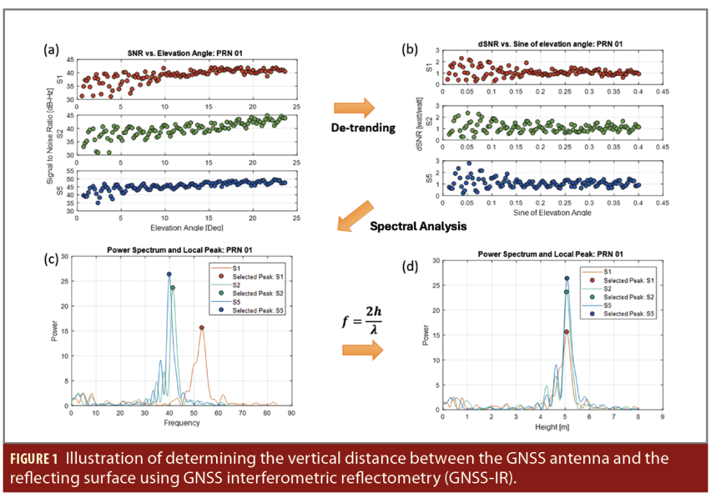
Figure 1 illustrates the overall workflow for estimating the vertical distance between an antenna and the reflecting surface by extracting multipath effects from the triple frequency GPS SNR signals, S1, S2 and S5.
In Figure 1a, the amplitude of SNR increases with the increasing satellite elevation angle, and the presence of oscillation pattern is also seen. To isolate the multipath effect, the trend is removed as shown in Figure 1b, denoted as detrended SNR (dSNR). The representing frequency of this oscillation can be found through a spectral analysis shown in Figure 1c. Each detrended SNR spectra have distinctive dominant frequencies with notable high-power spectrum, which presumably came from a planar reflector causing the multipath. The dominant frequency of each signal is converted to the vertical distance between the antenna and the reflector, that is the height of the surface, h, by taking into account the wavelength of each signal, λ. Consequently, the dominant peaks of three signals are aligned with similar heights as shown in Figure 1d.
While the theoretical framework of GNSS-IR suggests all frequencies should yield identical height measurements for a single reflector, practical observations often reveal slight misalignments, as seen in Figure 1d. This phenomenon arises because different signals—such as GPS L1 (1.575 GHz) and L2 (1.227 GHz)—interact with the reflecting surface differently. Factors like the antenna gain pattern and the surface’s electrical properties create a frequency-dependent scale error [14].
To ensure consistency, many researchers traditionally rely on a single frequency, often favoring GPS L2 because of its higher sensitivity to multipath effects [12]. While this approach provides stable returns, it disregards the redundant information available from modern triple-frequency GNSS signals.
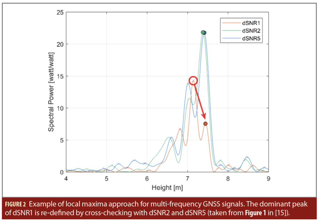
Our research [14, 15] takes a different path by leveraging the full spectrum of available observations (e.g., GPS L1, L2 and L5). We have found that while undetectable biases between frequencies do exist, their magnitude is generally smaller than the inherent observational noise of the GNSS-IR method as [14] reported the scale errors of L1 and L2 as 13 mm and 15 mm, respectively. By analyzing all three signals simultaneously, we can implement a “majority vote” logic to select the most reliable dominant peak. For example, Figure 2 illustrates the spectral power of detrended SNR (dSNR) for GPS L1, L2 and L5. In this instance, L2 and L5 show clear dominant peaks at a height of approximately 7.4 m, while L1 initially shows its strongest spectral power at 7.1 m. By examining the local maxima of the spectrum rather than just the single highest peak, we can identify a secondary peak that aligns with the 7.4 m measurement confirmed by the other two frequencies. This multi-frequency cross-verification significantly reduces the risk of outliers and improves the overall resilience of the monitoring system, especially in complex environments like the frozen Arctic.
A practical consideration in GNSS-IR is that retrieving the reflector height at a specific epoch requires a sufficient duration of time-series observations to characterize the oscillation pattern. This presents a challenge when monitoring dynamic surfaces, such as tidal water levels or moving ice, where the height is constantly changing. To capture this motion while maintaining high-precision results, we apply a sliding window to the dSNR data. This technique limits the observational period of the input signal to a specific temporal “snapshot” that accurately represents the surface height at that moment without sacrificing the frequency of the output.
In [16], we identified an optimal configuration for this sliding window by carefully balancing the sliding interval and the window width. While the interval can be adjusted based on the desired temporal resolution of the final data, the window width requires more precise calibration. It must be sufficiently large to capture the multipath-driven oscillations necessary for spectral analysis, yet narrow enough to prevent the “smearing” of dynamic surface behavior. Ultimately, the proper width is determined by the expected vertical distance between the antenna and the reflecting surface, ensuring the spectral peaks remain sharp even as the environment shifts. More exhaustive details on these parameter selections are provided in [15].
Monitoring Land-fast Ice in Alaska
GNSS-IR based tidal monitoring is particularly advantageous in extreme environments such as the Arctic and Antarctica. In these regions, accurate water level observations are vital, yet conventional tide gauges face significant operational hurdles. Because these instruments require direct contact with the water, their installation and maintenance are frequently compromised by harsh conditions and the periodic formation of ice. These limitations were addressed by using data from existing GNSS stations in Alaska to monitor tidal motion [15]. Our study identified and navigated specific high-latitude challenges, including reduced satellite visibility compared to mid-latitude regions and signal quality degradation caused by ionospheric scintillation. Despite these atmospheric and geometric constraints, we confirmed GNSS-IR serves as a robust and valid tide gauge alternative in the Arctic.
Because GNSS-IR measures the characteristics of the reflecting surface, the technique is applicable to monitoring both open water and ice surfaces. In Alaska, land-fast ice forms along the coastlines every autumn and persists until it melts away in the spring. Monitoring this nearshore ice is of critical importance for coastal communities, marine wildlife and regional navigation. Establishing seamless, year-round observations is therefore essential for coastal hazard preparedness and the safety of marine transportation.
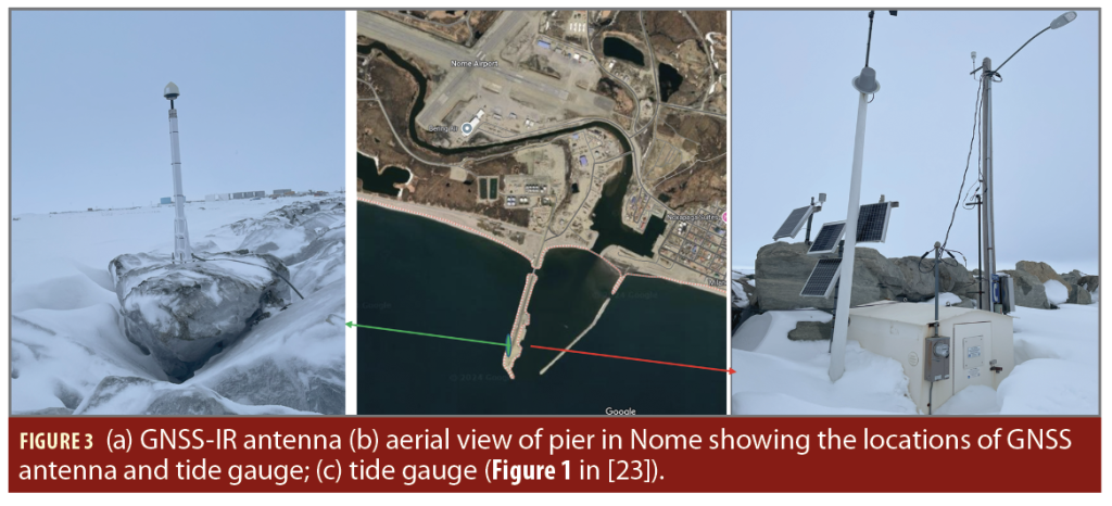
To address this need, our research group at Oregon State University (OSU) developed the GNSS-R Water-Ice observation system (GRWIS). The primary objectives of the GRWIS are threefold: to monitor tidal motion regardless of the presence of sea ice, to detect the onset of ice formation, and to assess the dynamic motions of land-fast ice. To validate the system’s performance, a GRWIS station was established in Nome, Alaska (64° 29′ 44.5″ N, 165° 26′ 20.0″ W), operating alongside a traditional tide gauge to provide a direct comparison of the GRWIS solutions.
The GNSS installation in Nome consists of a Septentrio PolaRx5S receiver and a single, upward-facing choke ring antenna mounted on a pier directly overlooking the ocean. This setup is strategically positioned opposite to an operational tide gauge, which is part of the National Oceanic and Atmospheric Administration (NOAA) National Water Level Observation Network (NWLON, Site ID: 9468756). Unlike the GNSS-IR system, which senses the surface remotely, this tide gauge is a contact-based sensor that is heated and structurally protected from the extreme open-ocean conditions of the Arctic. This specialized protection ensures a continuous record of water level estimations throughout the year, providing a reliable and high-fidelity benchmark against which the GRWIS solutions can be validated across both open-water and ice-covered periods.
Water Level Estimation Using GRWIS in Nome
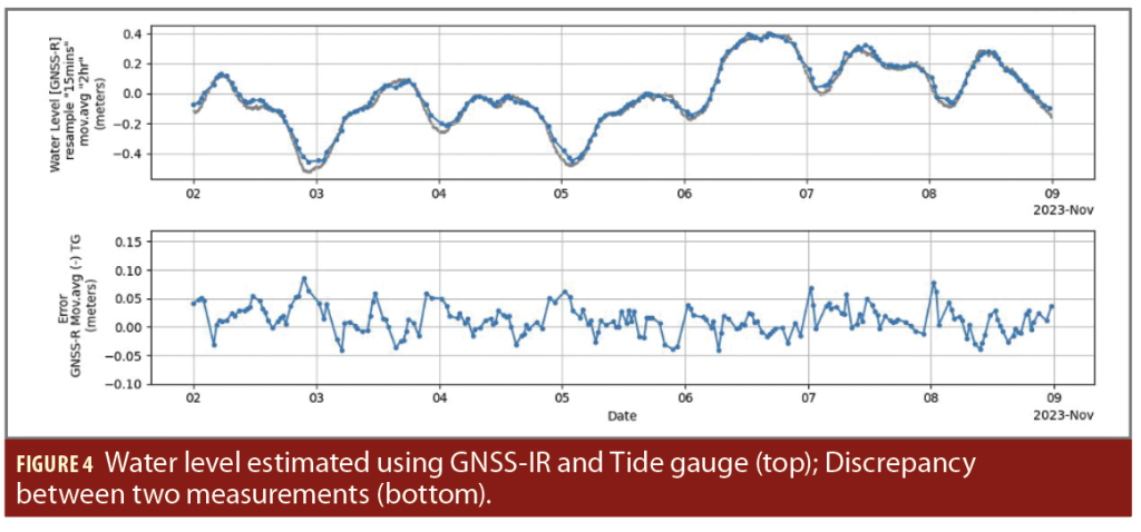
The experimental results from the Nome station demonstrate that GNSS-IR remains highly effective for water level estimation even under the rigorous constraints of high-latitude environments. While data acquisition and processing in these regions are often complicated by limited satellite geometry, ionospheric scintillation and extreme weather, our analysis showed strong agreement with the NWLON benchmark. Figure 4 illustrates a comparison between the GRWIS-derived water levels and the NOAA tide gauge during an ice-free period from November 2 to 8, 2023.
In the upper plot of Figure 4, the GNSS-IR based estimations (depicted in blue) closely track the ground-truth water levels provided by the NWLON tide gauge (depicted in grey). The lower plot quantifies the precision of the system, presenting the discrepancy between the two datasets. The residuals vary within a narrow range of approximately -5 cm to +5 cm, confirming the GRWIS system can achieve geodetic-grade accuracy for tidal monitoring despite the technical challenges inherent to the Arctic.
Sea Ice Detection
Monitoring sea ice using ground-based GNSS-IR is an emerging area of research, building on established principles of signal coherence and surface roughness. Early investigations by [17] in Disko Bay, Greenland, demonstrated a clear relationship between the number of coherent reflected signal observations and the presence of sea ice. This supported the earlier theoretical framework by [18], which posited that increased surface roughness on the open ocean significantly influences GNSS-R signal coherence. To quantify this, [19] introduced a damping coefficient derived from the attenuation of dSNR time series. While this coefficient includes unmodeled elevation-dependent effects, it serves as a proxy for reflector height variance and the physical state of the surface. More recently, [20] used GNSS interference frequencies to monitor sea ice in Finland. They noted that during frozen periods, the discrepancy between GNSS-IR height and mean sea level corresponds to the “total freeboard” (ice plus snow accumulation), which can be converted into ice thickness via hydrostatic balance equations.
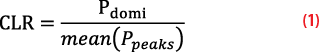
Our research group at OSU has advanced these methods by introducing a numerical indicator called the Confidence Level of Retrieval (CLR). The CLR is the ratio between the amplitude of the dominant spectral peak and the average amplitude of the remaining peaks in the SNR spectrum. It provides an intuitive measure of how clearly a single reflecting surface—such as calm water or flat ice—stands out against background noise or surface scattering.
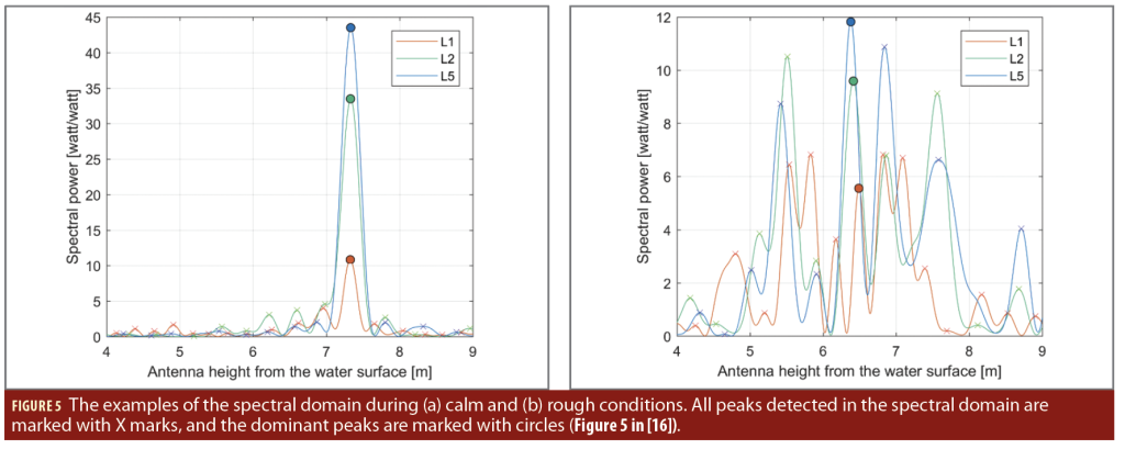
As illustrated in Figure 5, the spectral domain changes significantly based on surface conditions. In calm conditions (a), the dominant peak is sharp and unmistakable, resulting in a high CLR. Under rough conditions (b), the spectral power is distributed across multiple peaks (marked with “X”), lowering the relative strength of the dominant peak. We have found the CLR performs comparably to the damping coefficient used by [21] for monitoring wave heights, suggesting the CLR is a robust tool for characterizing the transition from turbulent open water to stable ice.
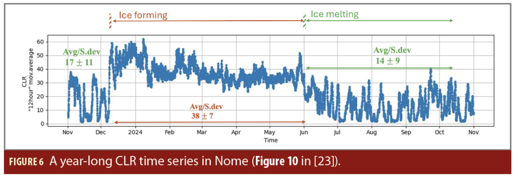
A year-long analysis of CLR data from Nome (November 1, 2023, to October 31, 2024) reveals a distinct seasonal signature that aligns with the formation and retreat of land-fast ice. During the ice-free period from November to early December, the moving average CLR remains relatively low at approximately 17 ± 9. Occasional dips below a value of 5 in this period correspond to rough sea states and high wave action. However, as land-fast ice stabilizes in mid-December, the CLR shifts dramatically, increasing to an average of 38 ±7. This high-confidence state persists until June 2024, when the spring melt commences and the CLR returns to its baseline ice-free average of 14 ± 9. This clear threshold behavior confirms the CLR is a highly effective metric for the automated detection of sea ice presence.
Spectral Analysis Using Continuous Wavelet Transform
To further analyze the complex frequency components of the GNSS-IR data, we employed the Continuous Wavelet Transform (CWT). Unlike the standard Fourier Transform or the Lomb-Scargle Periodogram, which decompose a signal into infinite sine waves and lose temporal localization, the CWT uses shifted and scaled versions of an original “wavelet”—an asymmetric, wave-like oscillation that begins and ends at zero [22]. This allows for the simultaneous extraction of instantaneous frequencies and their corresponding amplitudes over time, providing a clear advantage for monitoring non-stationary signals like those found in dynamic Arctic environments.
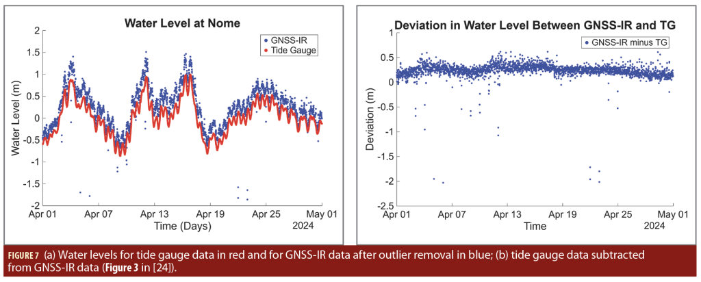
Our study specifically focused on data from April 2024, a period characterized by the simultaneous presence of sea ice and snow cover. Using estimation techniques, we compared GNSS-IR height measurements to the NOAA tide gauge benchmark after removing outliers exceeding three standard deviations (Figure 7a). A persistent offset was observed between the two datasets, largely attributable to snow accumulation on the land-fast ice. Because GNSS-IR signals reflect off the uppermost surface—in this case, the snow—the measurement represents the combined height of the water, ice and snow. In contrast, the heated, sheltered tide gauge measures the water level exclusively. By subtracting the tide gauge data from the GNSS-IR observations (Figure 7b), we effectively isolated the “deviation” signal, removing the dominant tidal motion to focus on higher-frequency surface dynamics.
The CWT output is visualized as a magnitude scalogram, where the x-axis represents time, the y-axis represents frequency, and the color intensity indicates the strength of the correlation between the signal and the wavelet. Within these scalograms, the Cone of Influence (COI)—indicated by dashed lines—marks the boundary where edge effects from the wavelet transform become significant. Data within the COI provides an accurate time-frequency representation, while results outside it are potentially influenced by the finite length of the time series.
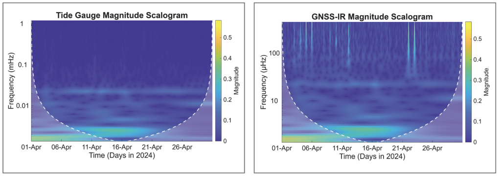
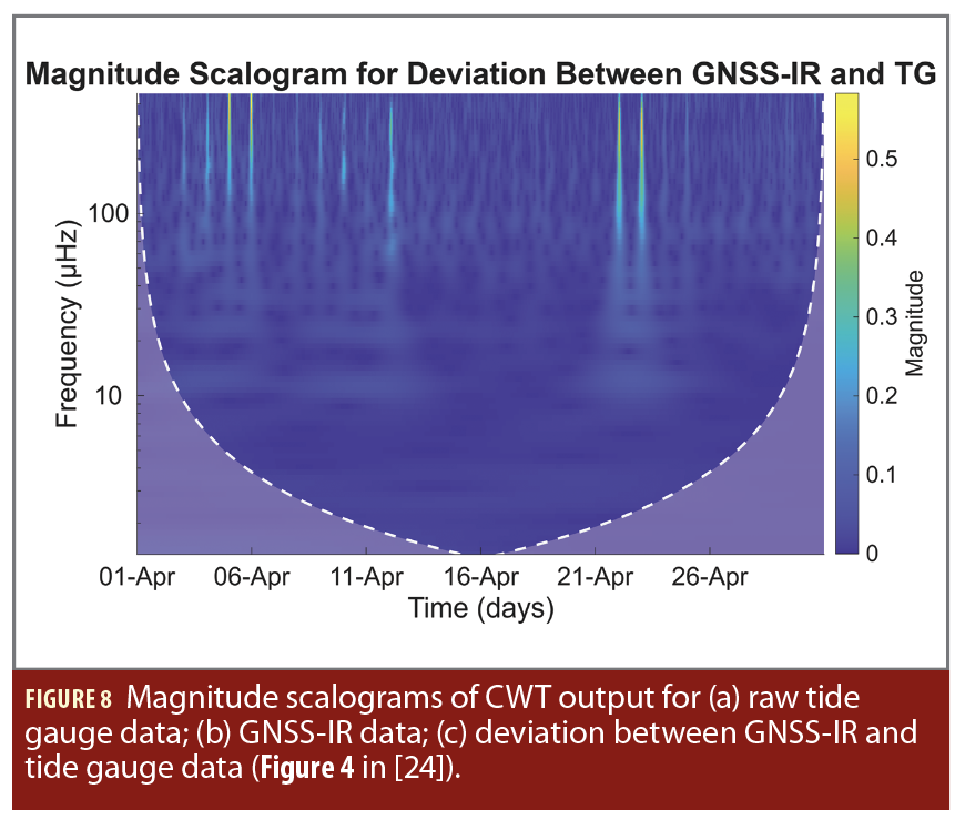
Analyzing the scalograms in Figure 8 reveals distinct differences. The tide gauge scalogram shows almost no high-magnitude regions at higher frequencies, consistent with a sensor protected from surface noise, while the GNSS-IR scalogram displays numerous high-magnitude “bright spots” at high frequencies. While some of this is inherent noise from multiple reflection points within the Fresnel zone, these signatures also capture non-tidal surface movements. By removing the low-frequency semidiurnal tidal components shown in Figure 8c, the remaining high-frequency signatures are isolated. While some outliers remain, these scalograms confirm GNSS-IR is capturing surface reflections beyond simple tidal oscillations.
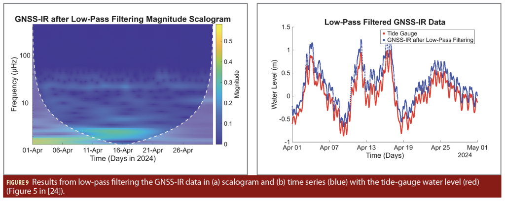
Through visual inspection of the scalograms, we identified a dominant energy band between approximately 2.0×10⁻⁵ Hz and 2.6×10⁻⁵ Hz. Using a bandpass filter, this region of the plot is isolated between 1.8×10⁻⁵ Hz and 2.8×10⁻⁵ Hz to calculate the period. The dominant period for the GNSS-IR data is 12.06 hours, and for the tide gauge data it is 12.83 hours, both of which align closely with the expected ~12-hour cycle of semidiurnal tides.
To isolate this tidal motion from the GNSS-IR data, we low-pass filtered at 2.6×10⁻⁵ Hz. After filtering, the majority of high-magnitude values at high frequencies are removed (Figure 9a). The low-pass filtered GNSS-IR water levels follow the tidal motion (Figure 9b). As shown in Figure 9, this filtering effectively removed the high-frequency magnitude peaks, resulting in a smoothed GNSS-IR water level time series that closely follows the tidal benchmark while maintaining the seasonal surface offset.
Detecting Snow Accumulation
Once land-fast ice is established, the reflecting surface effectively becomes a multi-layer system consisting of water, ice and accumulating snow. Because the GNSS-IR antenna captures reflections from the uppermost interface, its height measurements incorporate the total thickness of the snow and ice layers. In contrast, the heated and sheltered NOAA tide gauge continues to measure the water level exclusively. This disparity provides a unique opportunity to isolate snow depth by comparing the two datasets.
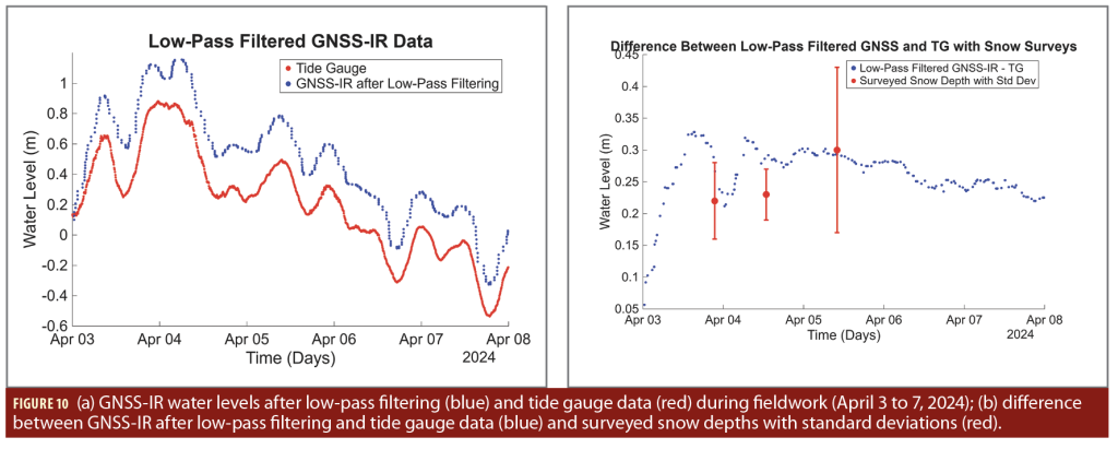
Figure 10a displays the low-pass filtered GNSS-IR water levels alongside the tide gauge data during the fieldwork period of April 3 to 7, 2024. At the beginning of this interval, the discrepancy between the sensors is near zero; however, the offset increases and fluctuates as the fieldwork progresses. We evaluated this difference by applying a six hour moving average to suppress uncharacterized high-frequency oscillations, revealing a clear trend in the surface elevation.
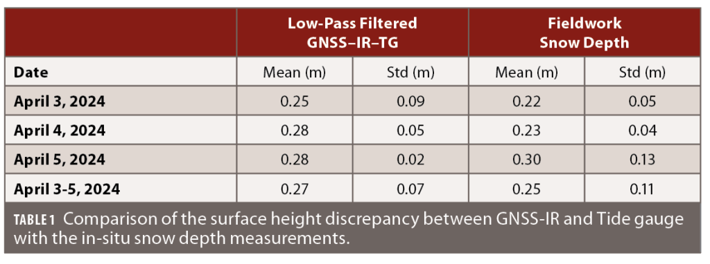
To validate whether this offset truly represents snow accumulation, we compared the GNSS-derived difference against in situ data from three snow surveys conducted during the fieldwork (Figure 10b). The GNSS-IR results summarized in Table 1 show reasonable agreement with the average snow depth and standard deviation from these physical surveys, supporting the hypothesis that the measurement offset is a direct proxy for snow depth.
Summary and Future Work
This study demonstrates that GNSS-IR is a versatile and robust tool for monitoring the Arctic’s complex, multi-layered environments. By using the GRWIS system in Nome, Alaska, we successfully established a method for independently estimating tidal motion, snow accumulation, and the dynamic signatures of land-fast ice from a single geodetic-grade receiver.
Our application of CWT proved instrumental in identifying the distinct frequency components within the reflected signals. By establishing precise cutoff frequencies, we were able to effectively low-pass filter the GNSS-IR data, isolating the semidiurnal tidal cycles from high-frequency surface noise. A key finding of this work is the characterization of the vertical offset between the remote GNSS-IR measurements and contact-based tide gauge data. By correlating these offsets with in-situ measurements, we have shown this discrepancy serves as a reliable proxy for snow depth, effectively turning a measurement “error” into a valuable environmental metric.
While the results are promising, the current validation of the snow-depth estimation is constrained by the relatively short duration of the April 2024 field campaign. A limited observational window for ground-truth data inherently restricts our ability to characterize the system’s performance across the full spectrum of Arctic weather events, such as heavy storm surges or rapid mid-winter melt-refreeze cycles.
Moving forward, we intend to expand our research to more precisely identify the specific spectral frequencies that correspond to snow depth and ice deformation. Future work will involve longer-term validation campaigns and the development of automated algorithms to separate snow accumulation from ice-loading events. By refining these multi-frequency GNSS-IR techniques, we aim to provide coastal Arctic communities with a maintenance-free, year-round solution for monitoring the increasingly unpredictable dynamics of land-fast ice.
Acknowledgment
The authors gratefully acknowledge the National Science Foundation (NSF) for its support of this research through the Arctic Observational Network (AON) EAGER grant #2321313. We also extend our gratitude to the local community in Nome, Alaska, and the NOAA Integrated Ocean Observing System (IOOS) for providing the critical benchmark data used in this study.
References
(1) Zakharenkova, I., Astafyeva, E., & Cherniak, I. (2016). GPS and in situ Swarm observations of the equatorial plasma density irregularities in the topside ionosphere. Earth, Planets and Space, 68, 1–11. https://doi.org/10.1186/s40623-016-0490-5
(2) Alfonsi, L., Cesaroni, C., Spogli, L., Regi, M., Paul, A., Ray, S., & others. (2021). Ionospheric disturbances over the Indian sector during 8 September 2017 geomagnetic storm: Plasma structuring and propagation. Space Weather, 19, e2020SW002607. https://doi.org/10.1029/2020SW002607
(3) Heki, K. (2006). Explosion energy of the 2004 eruption of the Asama volcano, central Japan, inferred from ionospheric disturbances. Geophysical Research Letters, 33, L14303. https://doi.org/10.1029/2006GL026249
(4) Heki, K. (2011). Ionospheric electron enhancement preceding the 2011 Tohoku-Oki earthquake. Geophysical Research Letters, 38, L17312. https://doi.org/10.1029/2011GL047908
(5) Park, J., Von Frese, R. R. B., Grejner-Brzezinska, D. A., Morton, Y., & Gaya-Pique, L. R. (2011). Ionospheric detection of the 25 May 2009 North Korean underground nuclear test. Geophysical Research Letters, 38, L22802. https://doi.org/10.1029/2011GL049430
(6) Luhrmann, F., Park, J., Wong, W. K., & others. (2025). Detection of ionospheric disturbances with a sparse GNSS network in simulated near-real time Mw 7.8 and Mw 7.5 Kahramanmaraş earthquake sequence. GPS Solutions, 29, 54. https://doi.org/10.1007/s10291-024-01808-2
(7) Luhrmann, F., Park, J., & Wong, W.-K. (2026). Ionospheric anomaly detection and source geolocation over open ocean with GNSS remote sensing. Journal of Geophysical Research: Space Physics, 131, e2025JA034460. https://doi.org/10.1029/2025JA034460
(8) Tahami, H., & Park, J. (2020). Spatial-temporal characterization of hurricane path using GNSS-derived precipitable water vapor: Case study of Hurricane Matthew in 2016. Geoinformatica: An International Journal, 7(1).
(9) Kang, I., & Park, J. (2021). On the use of GNSS-derived PWV for predicting the path of typhoon: Case studies for Soulik and Kongrey in 2018. Journal of Surveying Engineering, 147(4). https://doi.org/10.1061/(ASCE)SU.1943-5428.0000369
(10) Martin-Neira, M. (1993). A passive reflectometry and interferometry system (PARIS): Application to ocean altimetry. ESA Journal, 17, 331–355.
(11) Löfgren, J. S., Haas, R., Scherneck, H.-G., & Bos, M. S. (2011). Three months of local sea level derived from reflected GNSS signals. Radio Science, 46, RS0C05. https://doi.org/10.1029/2011RS004693
(12) Larson, K. M., & others. (2012). Coastal sea level measurements using a single geodetic GPS receiver. Advances in Space Research, 51(8), 1301–1310. https://doi.org/10.1016/j.asr.2012.04.017
(13) Benton, C. J., & Mitchell, C. N. (2011). Isolating the multipath component in GNSS signal-to-noise data and locating reflecting objects. Radio Science, 46, RS6002. https://doi.org/10.1029/2011RS004767
(14) Williams, S. D. P., & Nievinski, F. G. (2017). Tropospheric delays in ground-based GNSS multipath reflectometry—Experimental evidence from coastal sites. Journal of Geophysical Research: Solid Earth, 122, 2310–2327. https://doi.org/10.1002/2016JB013612
(15) Kim, S.-K., & Park, J. (2019). Monitoring sea level change in the Arctic using GNSS-reflectometry. In Proceedings of the 2019 International Technical Meeting of The Institute of Navigation (ION ITM 2019), January 28–31, 2019 (pp. 665–675). https://doi.org/10.33012/2019.16717
(16) Kim, S. -K., Lee, E., Park, J., & Shin, S. (2021). Feasibility Analysis of GNSS-Reflectometry for Monitoring Coastal Hazards. Remote Sensing.2021, 13, 976. https://doi.org/10.3390/rs13050976
(17) Semmling, A. M., Beyerle, G., Stosius, R., Dick, G., Wickert, J., Fabra, F., Cardellach, E., Ribó, S., Rius, A., Helm, A., Yudanov, S. B., & d’Addio, S. (2011). Detection of Arctic Ocean tides using interferometric GNSS-R signals. Geophysical Research Letters, 38, L04103. https://doi.org/10.1029/2010GL046005
(18) Soulat, F., Caparrini, M., Germain, O., Lopez-Dekker, P., Taani, M., & Ruffini, G. (2004). Sea state monitoring using coastal GNSS-R. Geophysical Research Letters, 31, L21303. https://doi.org/10.1029/2004GL020680
(19) Strandberg, J., Hobiger, T., & Haas, R. (2019). Real-time sea-level monitoring using Kalman filtering of GNSS-R data. GPS Solutions, 23, 61. https://doi.org/10.1007/s10291-019-0851-1
(20) Regmi, A., Leinonen, M. E., Pärssinen, A., & Berg, M. (2022). Monitoring sea ice thickness using GNSS-interferometric reflectometry. IEEE Geoscience and Remote Sensing Letters, 19, 2001405. https://doi.org/10.1109/LGRS.2022.3198189
(21) Roggenbuck, O., Reinking, J., & Lambertus, T. (2019). Determination of significant wave heights using damping coefficients of attenuated GNSS SNR data from static and kinematic observations. Remote Sensing, 11(4), 409. https://doi.org/10.3390/rs11040409
(22) Wang, X., He, X., & Zhang, Q. (2019). Coherent superposition of multi-GNSS wavelet analysis periodogram for sea-level retrieval in GNSS multipath reflectometry. Advances in Space Research, 65(7), 1781–1788. https://doi.org/10.1016/j.asr.2019.12.023
(23) Azeez, A., Park, J., & Mahoney, A. (2025). Preliminary results of nearshore ice and water level monitoring in Arctic using single antenna ground-based reflectometry. In Proceedings of the 2025 International Technical Meeting of The Institute of Navigation (ION ITM 2025) (pp. 216–228). https://doi.org/10.33012/2025.19982
(24) Bohn, J.J., J. Park, A. Mahoney, E. Fedders (2026), Monitoring the Dynamic Motion of Landfast Ice in Alaska Using GNSS-Interferometric Reflectometry (GNSS-IR), Proceedings of the 2025 International Technical Meeting of The Institute of Navigation, Anaheim, California, January, 2026.
Authors
Dr. Jihye Park is an associate professor of Geomatics in the School of Civil and Construction Engineering at Oregon State University (OSU). Before joining OSU, she worked as a post-doctoral researcher in Nottingham Geospatial Institute at University of Nottingham, UK. She holds a PhD in Geodetic science and surveying at The Ohio State University. Her research interests include GNSS positioning and navigation, Precise Point Positioning, Network Real-time kinematic, GNSS meteorology, GNSS-Reflectometry, and GNSS remote sensing for monitoring the earth environments, natural hazards, as well as artificial events.
Jaclyn Bohn is a graduate student at Oregon State University in the School of Civil and Construction Engineering studying geomatics. She received her bachelor’s degree in mathematics from the University of Utah. Her research interests lie in applications of GNSS-Reflectometry to monitor coastal areas.


