
This locality property makes it useful in modelling a variety of problems including mapping, visual-inertial odometry, motion planning, trajectory estimation and deep learning. The adoption of a GNSS factor graph may enable more seamless integration between GNSS and other sensor modalities.
A: Probabilistic modeling is a very important tool for any kind of estimation problem. Graphical models model known and unknown variables of a system using vertices in a graph and define edges between them to represent their relationship. Due to the inherent uncertainty in modelling a system, these relations are probabilistic. A factor graph connects many types of these graphical models like Markov Random Fields, Bayesian Networks, Tanner Graphs. The factor graph is defined as a Bipartite graph which has two types of vertices: one is the variable (i.e., the state vector) vertex which is to be estimated and another one is the factor vertex which encodes the constraints (e.g., a set of GNSS observations) applied to the variable vertices.
An edge can only exist between a factor vertex and a variable vertex. The factor vertices represent the local functions which depend on the variable vertices with which it shares edges. A common estimation problem in robotics uses the factor graph framework to estimate the unknown robot pose along with other parameters depending on the problem. This is achieved by solving the maximum-a-posteriori (MAP) problem, which maximizes the product of factors that are probabilistic constraints between states and measurements.
Factor graphs have been treated as an alternative framework for solving estimation problems and have proven very effective for specific applications including simultaneous localization and mapping (SLAM). This framework has attracted widespread use due to the flexibility of the approach and the ease of implementation granted through the availability of open-source graph optimization libraries like GTSAM and g2o.
While the factor graph framework has been proven beneficial for many applications, the framework can be used in an equivalent manner to (i.e., it is a generalization of) existing state estimation implementations (e.g., the Kalman filter and it many variants). To begin this comparison, we note that the factor graph ultimately encodes an objective function, which is solved through repeated relinearization via a non-linear optimization routine (e.g., Gauss-Newton, Levenberg–Marquardt). Previous work has demonstrated that iterating on the measurement update of extended Kalman Filter (EKF) and relinearizing the system models between iterations is equivalent to a Gauss-Newton optimization. This shows that, under a certain set of constraints, the factor graph operating in batch mode is equivalent to a backward-smoothing EKF that relinearizes system and observation models and iterates.
What Are The Advantages of Using a Factor Graph?
Factor graph optimization has some advantages over the standard non-iterated Kalman filter which may be valuable for certain applications. First, like any optimization problem, it uses multiple iterations to minimize a cost instead of just one iteration for each state as in a standard Kalman filter. Second, it also linearizes the nonlinear measurement model every iteration step for every state, unlike the single linearization performed by the standard Kalman filter. Factor graphs have also been shown to better exploit the time correlation between past and current epochs, which has been attributed to the batch nature of the estimation method.
In particular, when operating in a batch-mode, a factor graph would be equivalent to a forward filter and backward smoother after each measurement update. For GNSS/INS applications, these benefits have been supported by experimental results where factor graphs have been shown to perform better than an EKF in urban environments. It might appear that with accumulation of new measurements over a longer time, the batch estimation might lose real-time performance. But this is avoided through the exploitation of the sparseness of the graph. Furthermore, a sliding window approach can also be used to relieve computational cost. That is, instead of optimizing over all the states, only a local window of states are used (e.g., like a fixed-lag Kalman smoother).
The window size has been found to be crucial for good optimization results and can depend upon environmental conditions. Beyond fixed-lag smoothing, the incremental smoothing and mapping (isam2) formulation achieves real-time performance by converting the factor graph to the Bayes tree—the graphical representation of the square root information matrix (SRIF)—when a new constraint is added. The vertices of Bayes tree represent cliques of the factor graph states. Thus, only states contained within the same clique as the state with the new constraint need to be relinearized. Two of the authors used isam2 in a GNSS factor graph to show improved positioning performance over a traditional EKF-Precise Point Positioning (PPP) method. Another researcher applied factor graph optimization to the problem of both GNSS and GNSS-Real-time Kinematic (RTK) positioning and shows better performance than an EKF.
What Does a Factor Graph Applied to GNSS Look Like?
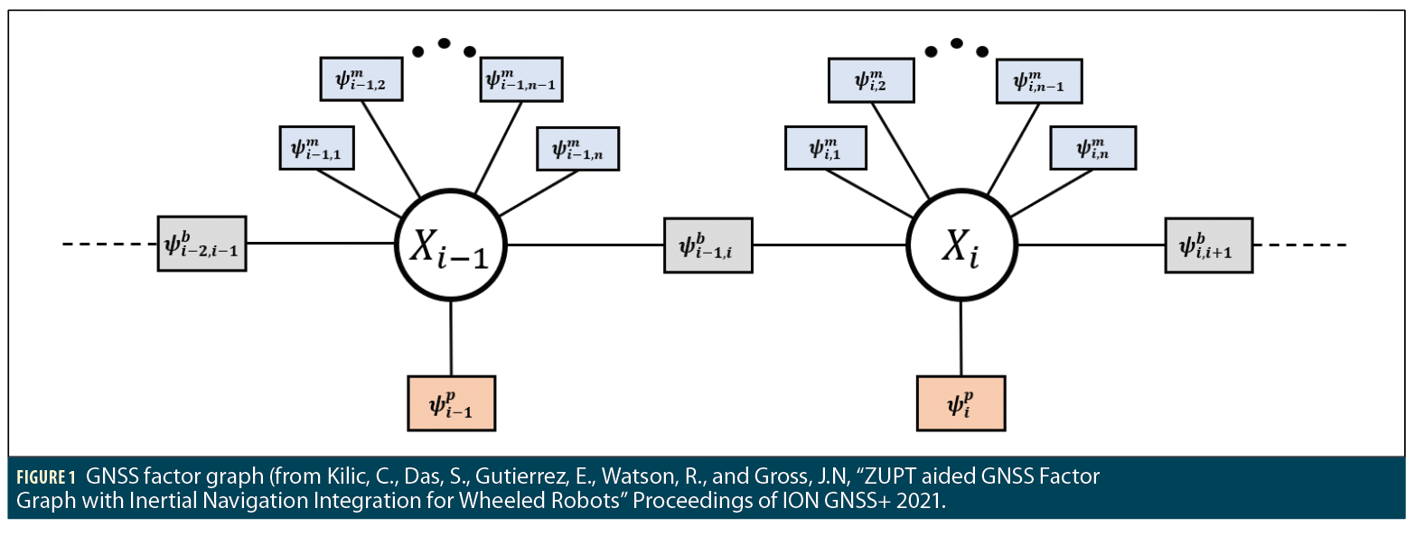
A detailed description of creating factors with GNSS observations is presented in a 2018 IEEE/ION/PLANS paper by two of the authors. The states commonly estimated in the GNSS factor graph are the receiver position, tropospheric delay, carrier-phase bias, and the receiver clock bias. Figure 1 provides a visual representation of the GNSS factor graph, where ψ represents any probabilistic constraint that might exist between the states and the measurements. In this specific implementation, ψp encodes the prior belief on each state, which depends on the specific data set and environmental characteristics. ψb is a motion constraint between two consecutive states along the trajectory which could, for example, incorporate motion data from an inertial measurement unit (IMU) or wheel odometry.
A common example of ψb used in GNSS/IMU navigation is the factor which uses IMU-preintegration to calculate displacement between the two factor-graph locations with multiple IMU measurements integrated between them. Finally, ψm are measurement constraint between a state and the measurements that were perceived from that state, for example GNSS pseudorange or carrier-phase measurements. To find the MAP estimate for the GNSS factor graph, we could find the set of states that maximize the product of factors. However, in practice, this optimization problem can be greatly simplified by employing the Gaussian noise assumption, which enables the conversion of the problem from maximizing the product of the factors to a non-linear least-squares problem where each component of the sum is a Mahalanobis cost, which represents sum of squares of the normalized residuals, as provided in Equation 1, where f(∗) is a mapping between states at different epochs and h(∗) is a mapping from the state space to the observation space.
What Are Methods for Robust Estimation Using Factor Graphs in GNSS?
As mentioned, the factor graph framework also makes it easy to add existing and new robust estimation methods which can help reduce localization error during spoofing attacks or large noise from multipath or atmospheric effects. The discussion below enumerates some of these robust methods applied to GNSS.
Switch constraints (SC), a lifted optimization methodology, defines an observation weighting function Ψ() that is a function of switch variables s, which is estimated in conjunction with the state parameters of interest. The SC method was initially developed for robust loop closure detection in SLAM and then extended to GNSS for multipath mitigation. When utilizing switch constraints, the pseudorange factor cost is expressed as a scaled version of the Mahalanobis cost between the predicted and actual measurement:
where the function Ψ is a linear function of the switch variable. Prior factors are added for each of these switch variables to stop the optimization from making all sk to zero. A transition factor can also be added to model the change between sk-1 and sk if the same satellite is observed at the next time step. These switch functions help in automatically de-weighting erroneous measurements (e.g., suspected multipath measurements) and are seen to perform better than computationally expensive ray-tracing methods.
In an extension of SC called dynamic covariance scaling (DCS), the switch variables are taken out of the optimization method and calculated separately using the residual, current measurement uncertainty and a prior switch uncertainty. After calculating sk, the information matrix associated with the GNSS observation factor is scaled by Ψ(sk)2.
Max-mixtures (MM) was also developed to tackle false loop closures using a Gaussian Mixture Model (GMM) but instead of the sum operator which is unsuitable for maximum likelihood when multi-modal uncertainty model is utilized, the objective function is converted to use the max operator, as shown in Equation 3.
The benefits of SC, DSC, and MM have been evaluated for GNSS factor graph applications with real-world data. Studies have shown the substantial positioning improvement that can be granted via the utilization of robust estimation techniques when conducting optimization with degraded GNSS observations.
To extend upon the max-mixtures work, two of the authors and colleagues proposed to learn the GMM during run-time based upon clustering of the observation residuals. Initially, this work was implemented in a batch framework; however, it was later extended to work incrementally, through an efficient methodology for incrementally merging GMMs.
M-estimators have also been recently tested within the GNSS framework in batch form and found to perform better than non-robust estimators. M-estimators assume a loss function that is different from the squared loss function. The squared loss function is highly sensitive to outliers since it grows aggressively for larger values of residuals. Thus, a group of loss functions were introduced which grow less aggressively than the squared loss function. The Huber cost function as provided in Equation 4 is one such function.
When the objective function is modified to utilize a m-estimator, the optimization problem takes a form as depicted in Equation 5.
where ri(x) is the residual for each measurement and σ is the scale parameter.
Increasing the ∆ parameter makes this function closer to the squared loss function. Equation 5 can be solved iteratively with weighted least-squares method. Selecting a suitable ∆ parameter is not straightforward, since it depends on the measurement noise statistics. Some M-estimators have a corresponding elliptical distribution to estimate the ∆ and the states in an Expectation Maximization (EM) framework. Another method jointly optimizes for the states and the parameters for computer vision applications.
A factor graph gives greater flexibility in the M-estimator application since it can help in de-weighting not only the current measurements but also changing the weights of the past measurements. It also can help is totally removing some past measurements if it is found to be an outlier later whereas in the Kalman filter, the contribution of past measurements cannot be changed in a real-time manner. Most graph optimization libraries also have built in functionality to use robust cost functions which is also helpful.
Finally, a robust estimation technique derived by Yang et al. unites the two well-known ideas from computer vision, the Black-Rangarajan Duality and Graduated Non-Convexity to iteratively solve the point-cloud registration problem using robust cost functions. According to the Black-Rangarajan Duality, equation 5 can be re-written as Equation 6:
where wi is the weight for the ith measurement and Φρ is a penalty term which depends on the weight and the robust cost ρ.
Graduated Non-Convexity (GNC) is a method to minimize a non-convex function f without facing the problem of local minima. The idea is to replace the function f with a surrogate function fµ whose convexity is controlled by the parameter µ. The optimization starts off with a convex form of fµ and µ is changed iteratively such that the nonconvexity increases. Uniting these two methods, Yang et al. solved two problems in Equation 5:
• avoiding local minima while optimizing a robust cost function
• convert equation 5 to a weighted least squares problem which is always easier to solve.
The similarity of this problem to GNSS should be obvious to the reader. Wen et al. shows importance of applying this robust estimation technique in GNSS factor graph in mitigating multipath effects in urban canyons. The batch nature of most of these robust estimation methods makes it suitable for use in a factor graph rather than an EKF.
What Are Potential Uses of Factor Graphs for the GNSS and Radio-Navigation Community?
The EKF has been the preferred choice for GNSS based state estimation due to their simplicity, computational efficiency, and the fact that GNSS observation models are well modeled by linear approximations and are often well characterized by Gaussian errors. Despite this, there may be situations in which the radio-navigation community can benefit from factor graph optimization.
For one, recent work has emphasized the potential use and benefits of signals of opportunity (SOP) in radio-navigation applications. SOP may include as cell phone signals and low-Earth orbiting satellites. Use of SOPs often includes a need to solve for an unknown or very uncertain transmitter location and clock offsets. Therefore, this class of problems shares many parallels with SLAM and may enjoy similar benefits from the use of a factor graph as recognized for visual or LIDAR based pose-graph SLAM.
Next, as discussed in the context of GNSS, many robust estimation techniques have been developed for use in factor graphs. For use of GNSS urban environments that is prone to multipath errors, these robust factor graphs may be beneficial. For example, the winning solution of the Google SmartPhone decimeter challenge, which included a variety of datasets collected different environmental settings, was indeed a factor-graph implementation.
Finally, factor-graph adoption may be beneficial simply because the factor-graph framework has become the standard state estimation paradigm within the robotics and autonomy communities (i.e., pretty much every sensor modality, other than GNSS, utilizes—and has shown the benefit of—the factor graph framework). The adoption of a GNSS factor graph may enable more seamless integration between GNSS and other sensor modalities. Integration of multiple information sources is a well-recognized key to any critical navigation system.
References
(1) D. Koller and N. Friedman, Probabilistic graphical models: principles and techniques. MIT press, 2009.
(2) B. J. Frey, F. R. Kschischang, H.-A. Loeliger, and N. Wiberg, “Factor graphs and algorithms,” in Proceedings of the Annual Allerton Conference on Communication Control and Computing, vol. 35. Citeseer, 1997, pp. 666–680.
(3) F. Dellaert, “Factor graphs: Exploiting structure in robotics,” Annual Review of Control, Robotics, and Autonomous Systems, vol. 4, pp. 141–166, 2021.
(4) F. Dellaert, M. Kaess et al., “Factor graphs for robot perception,” 2017.
(5) F. Dellaert, “Factor graphs and gtsam: A hands-on introduction,” Georgia Institute of Technology, Tech. Rep., 2012.
(6) G. Grisetti, R. Ku¨mmerle, H. Strasdat, and K. Konolige, “g2o: A general framework for (hyper) graph optimization,” in Proceedings of the IEEE International Conference on Robotics and Automation (ICRA), Shanghai, China, 2011, pp. 9–13.
(7) B. M. Bell and F. W. Cathey, “The iterated kalman filter update as a gauss-newton method,” IEEE Transactions on Automatic Control, vol. 38, no. 2, pp. 294–297, 1993.
(8) M. L. Psiaki, “Backward-smoothing extended kalman filter,” Journal of guidance, control, and dynamics, vol. 28, no. 5, pp. 885–894, 2005.
(9) W. Wen, T. Pfeifer, X. Bai, and L.-T. Hsu, “Factor graph optimization for gnss/ins integration: A comparison with the extended kalman filter,” NAVIGATION, Journal of the Institute of Navigation, vol. 68, no. 2, pp. 315–331, 2021.
(10) D. Wilbers, C. Merfels, and C. Stachniss, “Localization with sliding window factor graphs on third-party maps for automated driving,” in 2019 International Conference on Robotics and Automation (ICRA). IEEE, 2019, pp. 5951–5957.
(11) M. Kaess, H. Johannsson, R. Roberts, V. Ila, J. J. Leonard, and F. Dellaert, “isam2: Incremental smoothing and mapping using the bayes tree,” The International Journal of Robotics Research, vol. 31, no. 2, pp. 216–235, 2012.
(12) M. Kaess, V. Ila, R. Roberts, and F. Dellaert, “The bayes tree: An algorithmic foundation for probabilistic robot mapping,” in Algorithmic Foundations of Robotics IX. Springer, 2010, pp. 157–173.
(13) R. M. Watson and J. N. Gross, “Evaluation of kinematic precise point positioning convergence with an incremental graph optimizer,” in 2018 IEEE/ION Position, Location and Navigation Symposium (PLANS), 2018, pp. 589–596.
(14) W. Wen and L.-T. Hsu, “Towards robust gnss positioning and real-time kinematic using factor graph optimization,” arXiv preprint arXiv:2106.01594, 2021.
(15) C. Forster, L. Carlone, F. Dellaert, and D. Scaramuzza, “Imu preintegration on manifold for efficient visual-inertial maximum-a-posteriori estimation.” Georgia Institute of Technology, 2015.
(16) N. Su¨nderhauf and P. Protzel, “Switchable constraints for robust pose graph slam,” in 2012 IEEE/RSJ International Conference on Intelligent Robots and Systems. IEEE, 2012, pp. 1879–1884.
(17) C. Zach and G. Bourmaud, “Iterated lifting for robust cost optimization,” in BMVC, 2017.
(18) N. Su¨nderhauf, M. Obst, G. Wanielik, and P. Protzel, “Multipath mitigation in gnss-based localization using robust optimization,” in 2012 IEEE Intelligent Vehicles Symposium. IEEE, 2012, pp. 784–789.
(19) P. Agarwal, G. D. Tipaldi, L. Spinello, C. Stachniss, and W. Burgard, “Robust map optimization using dynamic covariance scaling,” in 2013 IEEE International Conference on Robotics and Automation. Ieee, 2013, pp. 62–69.
(20) E. Olson and P. Agarwal, “Inference on networks of mixtures for robust robot mapping,” The International Journal of Robotics Research, vol. 32, no. 7, pp. 826–840, 2013.
(21) T. Pfeifer, P. Weissig, S. Lange, and P. Protzel, “Robust factor graph optimization-a comparison for sensor fusion applications,” in 2016 IEEE 21st International Conference on Emerging Technologies and Factory Automation (ETFA). IEEE, 2016, pp. 1–4.
(22) R. M. Watson and J. N. Gross, “Robust navigation in gnss degraded environment using graph optimization,” in Proceedings of the 30th International Technical Meeting of the Satellite Division of The Institute of Navigation (ION GNSS+ 2017), 2017, pp. 2906–2918.
(23) R. M. Watson, J. N. Gross, C. N. Taylor, and R. C. Leishman, “Enabling robust state estimation through measurement error covariance adaptation,” IEEE Transactions on Aerospace and Electronic Systems, vol. 56, no. 3, pp. 2026–2040, 2019.
(24) ——, “Robust incremental state estimation through covariance adaptation,” IEEE Robotics and Automation Letters, vol. 5, no. 2, pp. 3737–3744, 2020.
(25) M. Bosse, G. Agamennoni, I. Gilitschenski et al., Robust estimation and applications in robotics.
(26) O. G. Crespillo, A. Andreetti, and A. Grosch, “Design and evaluation of robust m-estimators for gnss positioning in urban environments,” in Proceedings of the 2020 International Technical Meeting of The Institute of Navigation, San Diego, CA, USA, 2020, pp. 21–24.
(27) P. J. Huber, “Robust estimation of a location parameter,” in Breakthroughs in statistics. Springer, 1992, pp. 492–518.
(28) G. Agamennoni, P. Furgale, and R. Siegwart, “Self-tuning m-estimators,” in 2015 IEEE International Conference on Robotics and Automation (ICRA). IEEE, 2015, pp. 4628–4635.
(29) J. T. Barron, “A general and adaptive robust loss function,” in Proceedings of the IEEE/CVF Conference on Computer Vision and Pattern Recognition, 2019, pp. 4331–4339.
(30) H. Yang, P. Antonante, V. Tzoumas, and L. Carlone, “Graduated nonconvexity for robust spatial perception: From non-minimal solvers to global outlier rejection,” IEEE Robotics and Automation Letters, vol. 5, no. 2, pp. 1127–1134, 2020.
(31) M. J. Black and A. Rangarajan, “On the unification of line processes, outlier rejection, and robust statistics with applications in early vision,” International journal of computer vision, vol. 19, no. 1, pp. 57–91, 1996.
(32) A. Blake and A. Zisserman, Visual reconstruction. MIT press, 1987.
(33) W. Wen, G. Zhang, and L.-T. Hsu, “Gnss outlier mitigation via graduated non-convexity factor graph optimization,” arXiv preprint arXiv:2109.00667, 2021.
(34) K. Shamaei and Z. M. Kassas, “Receiver design and time of arrival estimation for opportunistic localization with 5g signals,” IEEE Transactions on Wireless Communications, 2021.
(35) ——, “LTE receiver design and multipath analysis for navigation in urban environments,” NAVIGATION, Journal of the Institute of Navigation, vol. 65, no. 4, pp. 655–675, 2018.
(36) J. J. Morales, J. Khalife, U. S. Cruz, and Z. M. Kassas, “Orbit modeling for simultaneous tracking and navigation using leo satellite signals,” in Proceedings of the 32nd International Technical Meeting of the Satellite Division of The Institute of Navigation (ION GNSS+ 2019), 2019, pp. 2090–2099.
(37) T. Suzuki, “First place award winner of the smartphone decimeter challenge: Global optimization of position and velocity by factor graph optimization,” in Proceedings of the ION GNSS+ 2021, 2021, pp. 2974–2985.
Authors
Shounak Das is a Ph.D. student at West Virginia University. He received a Master of Technology (M.Tech) in aerospace engineering from Indian Institute of Technology.
Ryan Watson completed a Ph.D. at West Virginia University and now works in the Autonomous Systems Group at Johns Hopkins Applied Physics Laboratory.
Jason Gross is associate professor and Associate Chair for Research in the Dept of Mechanical and Aerospace Engineering at West Virginia University, where he received his Ph.D.


