
The digital outputs of a four-channel antenna processing chain consisting of a four-element squared phased array and a 4-coherent channels front-end are processed to identify the presence of a jamming signal. The processing unit then implements a spatial filter to minimize jammer impact. The reconstructed signal is input to a COTS/SDR receiver designed to work in a typical railway environment.
By Cosimo Stallo, Pietro Salvatori, Andrea Coluccia, Radiolabs; Alessandro Neri, Massimo Massaro, University of Roma 3; Ernestina Cianca, Tommaso Rossi, Simone di Domenico, University of Rome Tor Vergata; Francesco Rispoli, Hitachi Rail STS; Massimiliano Ciaffi, RFI; Massimo Crisci, Christian Wullems, European Space Agency; and Giovanni Gamba, Qascom
GNSS has been selected as the key technology for modernization of the European Railways Train Management System (ERTMS). Its advantages—primarily cost saving, increased capacity and better allocation of resources—must be accomplished without compromising system safety. Radio frequency interference or jamming can degrade performance of a GNSS location determination system and can create a denial of service.
This article reports the results of a test campaign using a simulator to demonstrate the capabilities of an anti-jam platform: a four-channel antenna processing chain consisting of a four-element squared phased array and a 4-coherent channels front-end. The system can estimate the jammer direction of arrival, mitigate it, cleaning the useful signal from it and re-transmitting it to a COTS/SDR receiver.
The signal has been elaborated in post-processing with algorithms running on the platform. This approach exploits the possibility of injecting the front-end with signals that have the same phase shifts and attenuations that would have been experimented on the field with the given array geometry and element beam patterns.
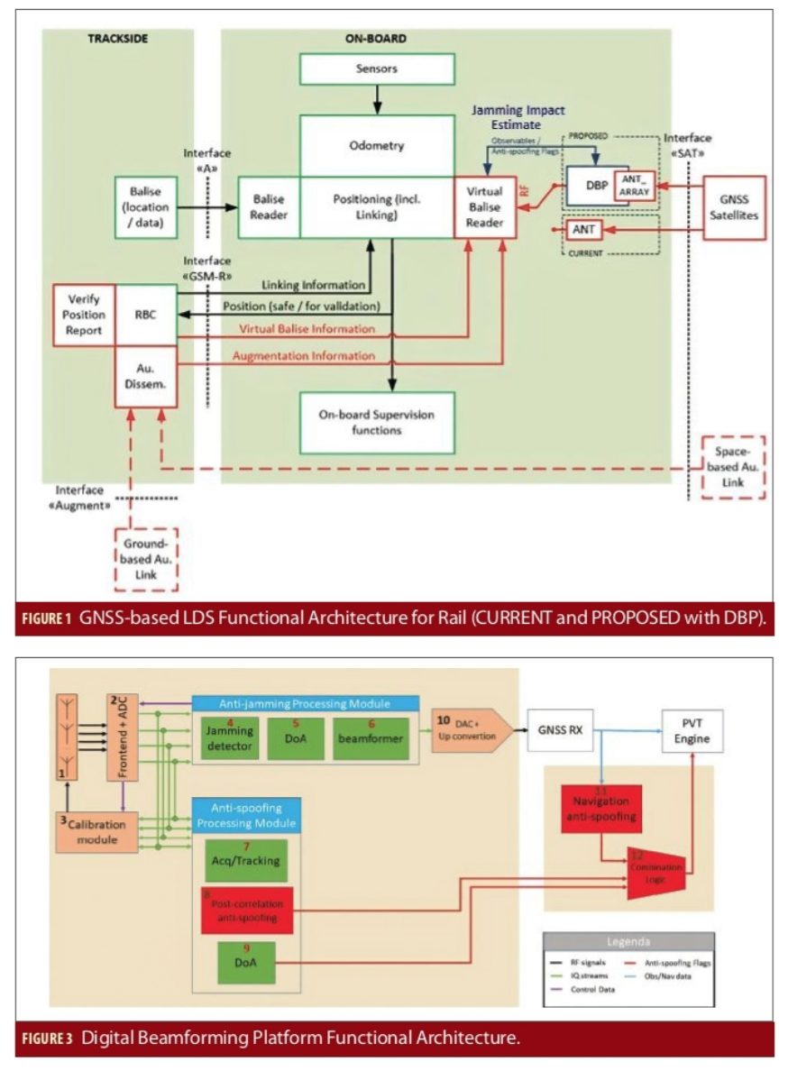
Figure 1 shows the operational concept of a digital beamforming platform (DBP) product to be used as a smart antenna connected to a GNSS receiver inside the virtual balise reader (VBR), increasing the PVT estimation resiliency against jamming and spoofing. Particularly, the main purpose of this system is to clean the signal from jamming, and to identify and exclude spoofing attacks.
Our goal is to improve the GNSS antenna bringing in the GNSS signal, by pre-processing RF signals before they enter the VBR. By means of sophisticated interference detection, estimation and mitigation techniques, the DBP aims at reducing the impact of jamming and spoofing signals that might arise in operational scenarios. The current form of the DBP is shown in green outlines.
Figure 1 also describes a potential proposed evolution derived from the DBP (indicated in red outlines), where the GNSS COTS antenna is replaced by a digital beamforming platform that is able to recreate a RF signal with mitigated interference, plus a set of ancillary anti-spoofing flags to be fed directly to the VBR.
The RF-to-RF DBP allows a complete drop-in replacement for the current GNSS antenna, minimizing the impact on VBR redesign. The VBR will only be able to accept and process digital anti-spoofing flags, but all the beamforming logic is contained in the DBP itself. The antenna array is external to the DBP. This approach is depicted in Figure 1-3. This approach (RF2RF) seems more practical, allowing a greater reuse of legacy VBR hardware and software.
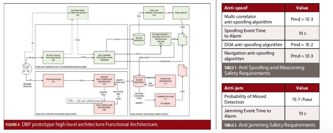
Figure 3 shows the functional architecture of DBP, while Figure 4 sketches the high-level architecture of the DBP prototype where the functions are mapped to software and hardware modules.
The safety requirements, deriving from apportionment by using FTA, in terms of probability of missed detection (Pmd) and Failure Rate (FR). Table 1-1 lists the DBP anti-spoofing and meaconing safety requirements. Table 1-2 describes the DBP anti-jamming safety requirements.
GNSS Antenna Array Design
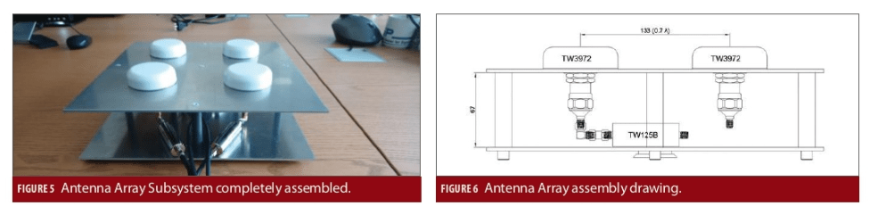
The antenna array subsystem is composed of four antennas and four in-line amplifiers. Each array element consists of an antenna providing triple band GPS L1/L2/L5, GLONASS G1/G2/G5, BeiDou B1/B2, Galileo E1/E5 plus L-band correction services coverage. The antenna provides superior multiipath signal rejection, a linear phase response, and tight Phase Centre Variation (PCV). It features a precision tuned, twin circular dual feed, stacked patch element. Figure 5 and Figure 6 show the two panels that protect the antennas connections and the in-line amplifiers. The two panels are separated by five PVC columns.
The characterization of the assembled 4 elements antenna array has been carried out in order to measure the radiation patterns of the antennas under test in the spherical near field system StarLab 18 GHz.
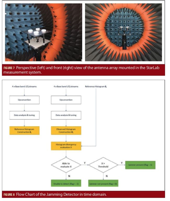
The assembled array has been mounted on the StarLab measurement system through a mechanical support, as shown in Figure 7. In this case, the in-line amplifiers have been removed for properly characterizing the intrinsic radiation characteristics of the array. Each element has an integrated low-noise amplifier and, thus, we expect to measure an embedded radiation pattern exhibiting a maximum gain around 37 dB. The power supply for the antennas was positioned outside the measurement system so as not to affect the radiation characteristics of the array.
GNSS Anti-Jam Chain Design
The jamming detection block uses a time-domain technique. The jamming detector algorithm is based on a “chi-square goodness of fit” test. This technique does not need a knowledge of the specific type of jammer. The algorithm requires a full characterization of received GNSS IF signals’ power density function (PDF) in absence of interference; this phase is called calibration one. This PDF can be modeled as a zero-mean white Gaussian process (being the CDMA GNSS signals buried inside the noise). In practice, a certain number K of PDF bins are measured during this calibration phase; this generates a histogram, called Ei (expected).
In the operational phase, the first step of the algorithm is to measure K bins of an incoming GNSS IF signal’s PDF, obtaining a histogram called Oi (observed). The chi-square test statistic is defined as:
The test statistic can be considered as an instance of a random variable, Tχ(x), that is χ2-distributed. The test is performed evaluating the following probability (called p-value):
If pm=1, the two histograms are identical; if pm=0 then the histograms are different.
The decision on the presence of a jammer is performed fixing a threshold, pα. If the p-value is higher than the threshold, it is posited that no jammer is present (jamming presence flag is set to 0), otherwise, the presence of a jammer (jamming presence flag is set to 1) is posited.
Thanks to the antenna array, the “chi-square goodness of fit” test can be performed individually over each antenna. The final decision about the jamming detection is taken by using the average p-value computed as the mean of the p-values obtained from the 4 antennas. This choice can improve the performance of the jammer detector thanks to the spatial diversity provided by the 4 antennas. The jamming detector block performs the following operations:
• Collection of the 20 ms of samples;
• Adaptation of the number of bins and edges as function of the input signal;
• Construction of the histogram
(Ei or Oi);
• Jamming detection flag generation: it performs a χ2 goodness of fit test and takes a threshold value as input.
Figure 8 shows the flow chart of the jamming detector in time domain.
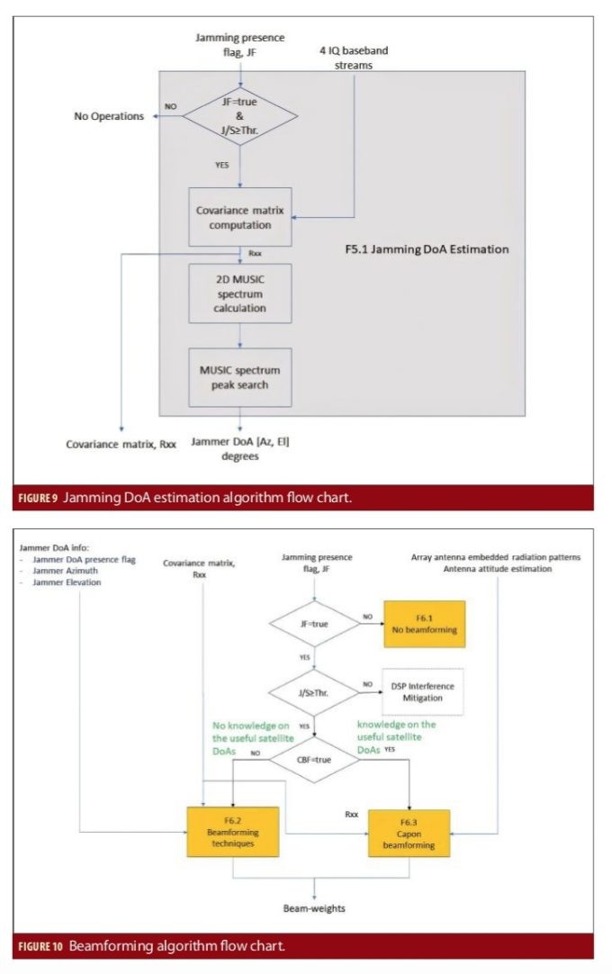
The DoA jamming estimator is responsible for the estimation of the DoA of the jammer. This block is activated only if the jamming presence flag is true and J/S>=Threshold. This block is based on MUltiple SIgnal Classification (MUSIC) algorithm. It is a subspace method that exploits the structure of the received data. Jammer DoA is estimated finding the associated steering vectors that are orthogonal to the noise subspace and contained in the signal subspace. Figure 9 displays its functional block flow chart.
Module #6 is in charge of signal beamforming and jamming mitigation through beamforming algorithm (Beamforming and Pre-correlation Interference mitigation). If jamming presence flag is true and J/S>=Threshold, jamming mitigation is activated.
Two main options are envisaged, which can be selected according to the specific application scenario by setting the Boolean flag CBF:
Option #1 (CBF=false): the knowledge of the useful satellite DoAs cannot be guaranteed. In this case, only beamforming techniques that do not pose constraints of the useful signals’ directions can be used, such as simple null steering or blind techniques such as Power Minimization (PM). Null steering is a simple option: when placing the null, there is no guarantee that useful satellite signals are “protected” and their SNRs could be strongly degraded. This is why the PM option is also kept. Particularly, if the DoA estimation module has been able to determine the jammer azimuth and elevation, the null-steering technique is selected; instead, if the jammer DoA is not available, the power minimization technique is used.
Option #2 (CBF=true): in this case, the DoAs of useful satellite signals are available and Capon beamforming can be applied. This algorithm minimizes the beamformer output power; linear constraints are used to control the antenna directivity towards K useful sources that will be “protected” (where K is lower than array antenna elements). These constraints are defined using useful satellites DoA from GNSS almanac.
Array antenna embedded patterns are corrected using array attitude information. Corrected embedded patterns are an input for Capon algorithm.
The functional block flow chart is reported in Figure 10 and Figure 11. Three options have been foreseen:
• No active beamforming: the beamweights are set to [1, 0, 0, 0], where 1 is associated to the reference antenna.
• Power Minimization (PM)/Null Steering (NS) in the case of no knowledge on the useful satellites DoAs.
• Capon Beamforming in the case of knowledge on the useful satellites DoAs.
Module #10 is composed of a digital to analog converter (DAC), an up-converter and a RF transmitter at L1 GPS and E1 Galileo. The I/Q stream received after the beamforming is up-converted to RF and it is converted into an analogue signal by using a DAC. The obtained signal is then transmitted in output of the DBP.
Jammer Detector Performance
Jammer detector performance has been evaluated in terms of probability of false alarm and missed detection, with respect to different jammer/signal ratios (JSRs). GNSS signals have been generated by using a GNSS/GPS simulator and received by using an SDR platform simulating an antenna array made up of 4 patch antennas at 0.7λ.
GNSS signals have been sampled at 8 Msps for about 40 seconds, where each sample represents a complex baseband IQ sample quantized by using 2 bytes for both the real and imaginary part. All GNSS signals have been weighted for the complex embedded antenna array radiation pattern.
The simulated jammer scenarios are the following:
• GNSS signals in absence of any jammer signals and in presence of multipath propagation.
• GNSS signals in presence of a jammer signal with JSR=10dB and multipath propagation.
• GNSS signals in presence of a jammer signal with JSR=30dB and multipath propagation.
• GNSS signals in presence of a jammer signal with JSR=10dB and in absence of multipath propagation.
• GNSS signals in presence of a jammer signal with JSR=20dB and in absence of multipath propagation.
The jammer detector algorithm has been calibrated by using GNSS signals in absence of any jammer signals, and the following parameters have been chosen:
• Detection period=20 ms
• Number of bins=16.
• Level of significance=10-4.
The p-value over time computed by the jammer detector algorithm for the GNSS signals collected in absence of any jammer signals is always above the level of significance, fixed at 10-4 during the calibration phase, except for one detection period, which causes a single false alarm event over all the acquisition interval. The plot at the bottom half of Figure 12 shows the result provided by the Chi-square goodness of fit test over time, expressed in terms of the test hypothesis I.
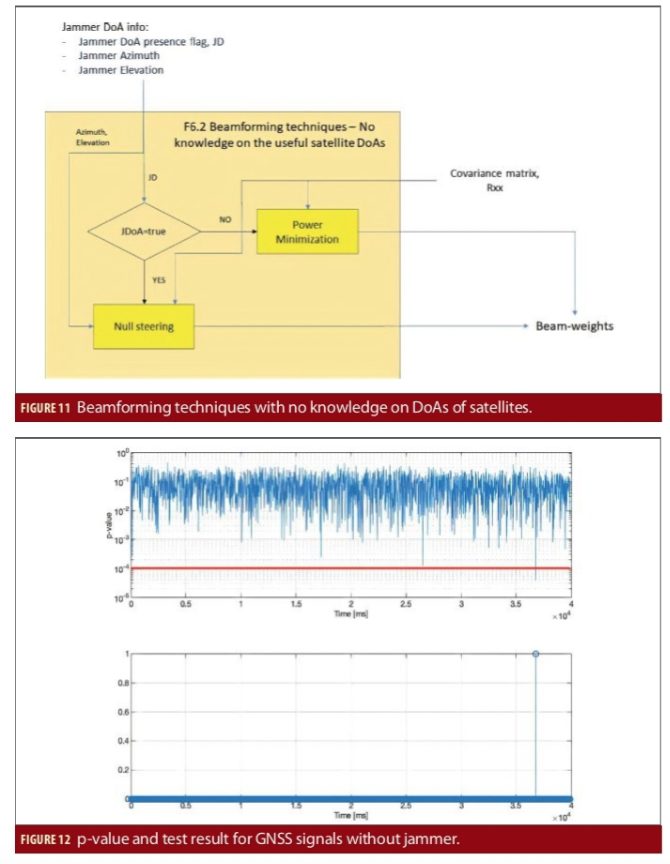
In the jammer detection scenario, the null hypothesis, i.e. I=0, is a hypothesis that says there is no statistical difference between the histogram estimated during the calibration phase and the one measured in a detection interval during the test phase, which means that no jammer is present in the target time slot. Conversely, the alternative hypothesis, i.e. I=1, is a hypothesis that says there is statistical difference between the compared histograms, which means that the test has detected a jammer within the detection interval processed. From the plot at the bottom of Figure 12, it can be noted, according to the p-value reported above, how the null hypothesis is accepted for all the time, except for one case, which corresponds to the detection interval where the p-value goes below the threshold of the test. The probability of false alarm evaluated over this dataset is Pfa=0.0005% (10-6).
The probability of missed detection has been evaluated by using the same calibration settings and data used to evaluate the probability of false alarm, and the GNSS datasets characterized by the presence of a jammer signal. The probability of missed detection evaluated over the 4 datasets is 1-Pd=0%. This means that the jammer is always detected by the algorithm. In this case, figures showing the p-value over time computed by the detection algorithm are not reported since the p-value is constantly equal to 0.
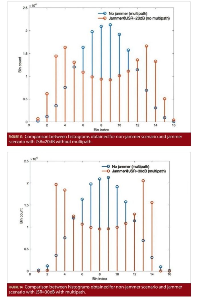
This excellent result is due to the fact that the probability density function, and hence also its histogram, of the received signal in presence of jamming is significantly different from the probability density function of the GNSS signal in absence of any interfering source. This means that the Chi-square test in presence of jamming always provides very high value of the statistical metric, which leads to a p-value equal to 0 and therefore to a correct detection of the jammer.
For a better understanding of this result, it is useful to show a comparison between the histogram constructed during the calibration phase and the histogram constructed by using the data received within a detection interval for a jammer scenario. The comparisons for some jammer scenarios, which are JSR=20 dB without multipath, and JSR=30 dB with multipath are shown in Figure 2.2.1.1-2 and Figure 2.2.1.1-3, respectively.
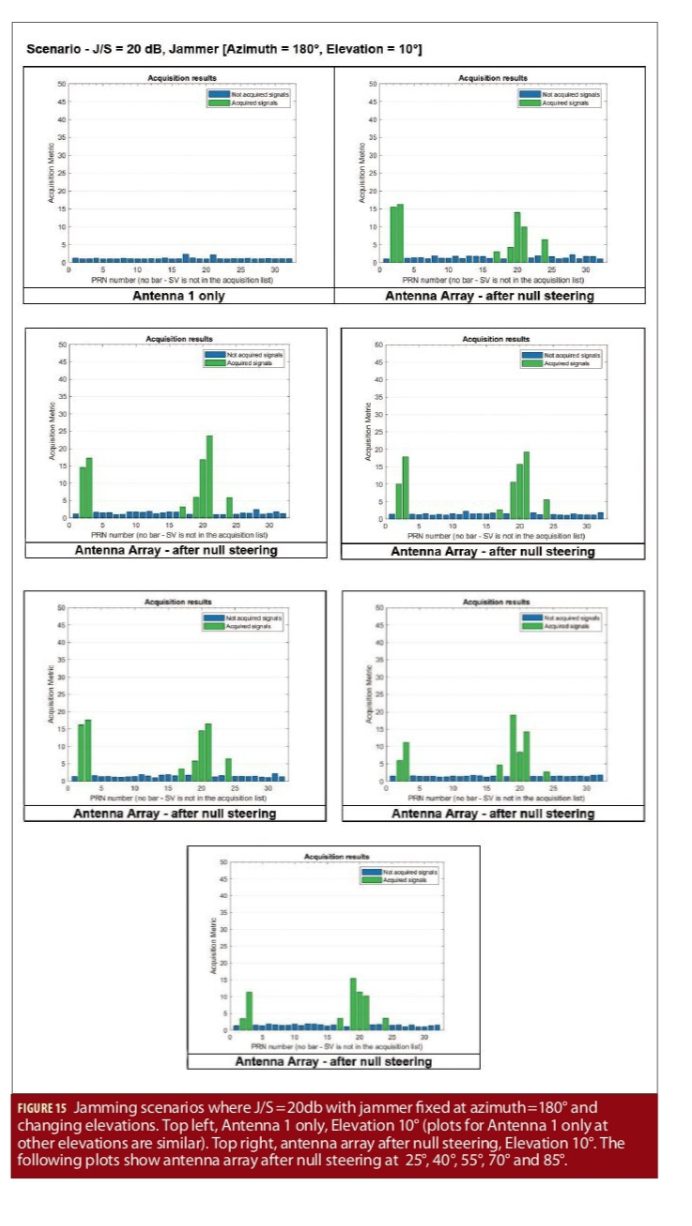
An analysis of impact of beamforming operation on the I/Q beamformed signal up-converted at RF has been evaluated through a SDR receiver in terms of useful signals acquired and tracked by receiver after null steering (considering the antenna array) in presence of a jammer with regard to a classic solution based on single antenna and no beamforming.
The analysis of the signal synthesis module has been carried out generating a set of synthetic GNSS I/Q streams. These streams have been generated covering the sky with a step of 45° in Azimuth (from 0° to 315°) and 15° in Elevation (from 10° to 85°). Those generated data are then affected by a chirp jammer with 3 different levels of power in terms of J/S: 10 dB, 20 dB and 30 dB. The I/Q streams are then elaborated by the entire anti-jamming chain (Jamming detector, DoA estimation, Beamformer) by using the null-steering approach.
After the spatial filtering, the data are up-converted to IF and analyzed by the Borre’s SDR tool. More in details, for each dataset has been evaluated which satellite passed the acquisition process before and after the DBP. The IF frequency selected is 10 MHz with a sampling frequency of 40 MHz. The results are reported below. According to them, the beamformer (F6.2 and F6.3) are effective when J/S is higher than 10dB. When J/S is equal to 10 dB, the beamformer (F6.2 and F6.3) is effective when the elevation in LoS between jammer and DBP is higher than 10 degrees. Figure 16 represents the scenario where J/S=20 dB with Jammer fixed at Azimuth=180° and changing elevation.
Conclusion
The work shows the performance in terms of anti-jam capabilities of a digital beamforming platform designed for rail scenarios and able to act as a smart antenna cleaning potential jammers and re-transmitting the useful GNSS signals directly to the GNSS receiver inside the VBR. DBP is necessary means to pave the way of secure receiver with railways security standards.
Acknowledgments
This work is funded under the Contract ESA GSTP 6-2 “Digital Beamforming for Rail”. Special thanks for their support to Christian Wullems and Massimo Crisci from ESA.
An earlier and more extensive form of this work was presented at ION ITM 2020; see www.ion.org/publications/browse.cfm.
Manufacturers
The antenna array consists of Tallysman TW3972 antennas. The simulator was a Spirent GSS9000, with the SDR platform NI 2955 simulating an antenna array


