GNSS signals are vulnerable to interference due to being extremely weak when received on Earth’s surface. Therefore, even a low-power interference signal can easily disrupt the operation of commercial GNSS receivers within a range of several kilometers.
GNSS signals are vulnerable to interference due to being extremely weak when received on Earth’s surface. Therefore, even a low-power interference signal can easily disrupt the operation of commercial GNSS receivers within a range of several kilometers.
Interference signals can originate from various sources, such as TV transmitters, radio amateur equipment, and personal privacy devices (PPDs), which are easily available despite being illegal. Although PPDs are intended to deny GNSS signals within a few meters, they often transmit excessive jamming power that interrupts signals considerably beyond personal range. In some cases, the illegal usage of high power PPDs has interrupted the operation of critical infrastructure systems such as airport landing equipment. (See the article by J. C. Grabowski in the Additional Resources section near the end of this article.) Consequently, anti-interference mechanisms are becoming increasingly important to develop for modern GNSS applications.
Several types of RF interference signals can adversely affect GNSS operations and can in general be categorized into different groups, such as intentional and unintentional, wide-band, partial-band, and narrow-band interference. Single-tone and chirp interference signals are two of the most important intentional interference generated by PPDs. These are discussed in further detail in the articles by R. Bauernfeind et alia (2014) and R. H. Mitch et alia listed in Additional Resources.
Interference countermeasure methods are generally divided into two categories, namely pre-despreading and post-despreading techniques. The pre-despreading methods attempt to detect the presence of interference signals and characterize them before the received signals are fed to correlator branches in a receiver.
As these methods usually work on the raw received samples, their associated processing rate is much higher than that of post-correlation methods. Pre-despreading interference detection and characterization techniques are more efficient and usually detect interference signals faster than post-despreading methods. Post-despreading techniques usually analyze the carrier-to-noise-density (C/N0) variations of the received signals after being tracked by the receiver and is measured in terms of the effective degradation in GNSS receiver performance caused by interfering signals.
Prior research has proposed several interference detection methods each of which focuses on a specific feature of interference signals such as power content, spectral/spatial power density, or signal amplitude distribution. However, limited work has been done to assess the efficacy of these techniques from a practical perspective.
Several approaches have been proposed for detecting the presence of interference signals. An energy detector is the simplest and the most commonly used pre-despreading interference detection technique. This method measures the received signal energy during a finite interval and compares it with a predefined decision threshold. However, a spectrogram is the optimal detector for periodic signals such as narrowband continuous wave (CW) interference. The performance of this method can exceed that of the energy detector for the case of narrowband interference signals.
Some interference detection techniques focus on analyzing the statistical distribution of the received sample set and try to detect the presence of jamming signals based on the histogram deviation from the expected Normal distribution. Another analytical method for GNSS interference detection assesses the performance of Chi-square Goodness of Fit (GoF) methods.
This article describes various types of interference signals commonly generated by PPDs. We then analyze the effective C/N0 of GPS L1 and Galileo E1 signals in the presence of these types of interference signals. The article next reviews various pre-despreading approaches to detecting interference to GNSS signals and compares their performance in terms of probability of detection and false alarm, detection latency, and computational/hardware complexity. These detection techniques include time, frequency, and space domain processing methods.
We used a variety of simulations to evaluate the performance of the detection techniques for different interference types and power levels. The results show that, using a proper combination of interference detection methods, it is possible to detect different types of interference signals even if they are not powerful enough to significantly deteriorate the GNSS receiver performance.
Common Interference Signals
This section reviews two of the most common interference signals.
Narrowband Continuous Wave (CW) Interference. This category of narrowband interference refers to a single sinusoidal tone within a GNSS frequency band and can be represented as
JCW(t) = Acos(2πfcwt + φ0) (1)
where A is the amplitude, fcw is the interference frequency, and t is the time. φ0 is the initial phase of the interference signal. For CW interference, the signal frequency is assumed to be time invariant.
Chirp Interference. This category of continuous wave interference consists of a sinusoidal waveform whose frequency repeatedly sweeps across a certain bandwidth. The mathematical representation of this signal can be written as
Jchirp(t) = Acos(2πfchirp(t) + φ0) (2)
where fchirp(t) is the instantaneous frequency of chirp signal at time t and is commonly a linear saw-tooth function of time. This type of interference is the most common signal transmitted by low-cost PPD jammers. The frequency span is commonly between 7 and 60 megahertz, and the sweep time is on the order of tens of microseconds. This type of interference can be considered a wideband interference because it sweeps the whole L1/E1 frequency band several times during the coherent integration time of a typical receiver.
Gaussian Noise Jammers. The source of this type of interference propagates wideband noise across the whole frequency band of the target GNSS system. The wideband noise jamming signals cannot be discarded via notch filtering because the power content is distributed across all frequency components.
System Model
For the case of a single antenna receiver, the interference-contaminated received signal can be written as
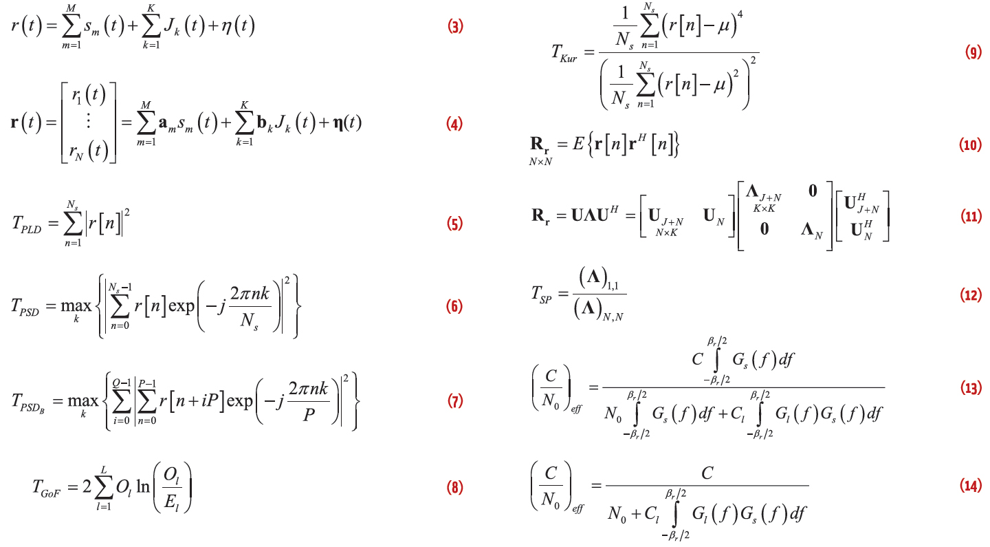
Equation (3) (see inset photo, above right, for all equations)
where sm(t) is the received signal from the mth satellite, Jk(t) is the jth interference component, and η(t) is the additive white Gaussian noise (AWGN) component. M and K are the total number of GNSS and jamming signals. sm(t) is a spread spectrum signal with a very low power spectral density which is buried under the noise floor before the despreading process. Jk(t) could be any type of narrowband or wideband interference signal whose power is considerably higher than the ambient noise.
Drawing on the work described in the article by S. Daneshmand cited in Additional Resources, for the case of an N-antenna receiver the received signal model can be written as
Equation (4)
where η(t) is an N•1 complex AWGN vector with covariance matrix σ2I where I is an N•N identity matrix. am and bk are steering vectors of GNSS and interference signals. These vectors incorporate all spatial characteristics of the antenna array for GNSS and interference signals and are a function of array geometry and angles of arrival (AoA) of incident signals.
Review of Interference Detection Methods
This section discusses some of the most prominent interference detection methods and their advantages and limitations.
Power Law Detector (PLD). The power law detector is the simplest and most commonly used approach for interference detection. This method measures the received signal energy during a finite time interval and compares it with a predefined decision threshold. The test statistic for PLD is written as
Equation (5)
where r[n] is the digitized version of the received signal, r(t), sampled at nTs instant, and Ns is the number of samples over which the power calculation is performed.
PLD is optimal for detection of white Gaussian interference signals embedded in AWGN when the expected values of noise power are already known. However, defining an accurate detection threshold practically may become challenging in the case of unknown statistical features of ambient noise. One approach for solving this problem is observing a clean data set and setting the detection threshold based on its statistical features as discussed in the article by S. Atapattu et alia.
Power Spectral Density (PSD) Analysis. Partial band and narrowband interference signals are more observable in the frequency domain using a spectrogram operator. The spectrogram is the optimal detector when the interference is a sinusoid of unknown amplitude, phase, and frequency. Herein, the detection test statistic can be written as
Equation (6)
where exp(.) represents an exponential function and j is the square root of –1. Ns represents the number of samples over which the Discrete Fourier transform (DFT) is calculated and k ranges from 0 to Ns–1. An interference signal would be detected if ΓPSD exceeds a pre-defined detection threshold. The detection threshold is assumed to be determined based on a clean assessment window and a pre-determined false alarm probability.
For longer data intervals, we can calculate an averaged spectrogram such as Bartlett’s spectrum:
Equation (7)
where Q and P represent the number of averaging and the number of samples used in the DFT process, respectively. Herein, the total number of temporal samples is equal to Ns=PQ. In a method described in the paper by F. M. Ahmed et alia, the threshold can be calculated by considering the variance of an interference-free part of the data.
Probability Density Function (PDF) Analysis. In the absence of interference signals and prior to the despreading process, thermal noise is the dominant component. Therefore, interference-free signals are expected to obtain a zero mean Gaussian distribution. However, in the presence of non-Gaussian interference signals, the distribution deviates from a Normal distribution.
The following sections describe two tests to detect this deviation:
- Chi-Square Goodness of Fit (GoF). This test compares the histogram of received samples with the interference-free signal histogram. The algorithm involves assigning the data values into discrete amplitude bins and counting the number of samples belonging to each bin. The bin counts are used to form the following Chi-square G-test statistic:
Equation (8)
where L is the number of histogram bins. Ol and El are the observed and expected sample counts in the lth bin normalized to the total sample (Ns). ln(.) represents the natural logarithm function. If the number of samples Ns is large, the test statistic can be modeled by a Chi-square distribution with L–1 degrees of freedom.
In this test, the calculation of El could be based on an interference-free assessment window or based on a Normal distribution that follows the mean and variance of the observed sample set. For this article, we call the former case trained GoF or (GoFT) and the latter non-trained GoF or GoFNT.
- Kurtosis Test. Kurtosis is a statistical parameter that describes the shape of a distribution. It denotes how peaked a distribution is compared to a Normal distribution. The kurtosis of a distribution is defined as the ratio of its fourth moment to the square of its second moment:
Equation (9)
where Ns is the number of samples under analysis and μ is the mean of the observed sample set.
The theoretical value of the kurtosis for a normal distribution and a sufficiently long sample set is three and is independent of the value of the signal variance. However, in the presence of non-Gaussian interference, the kurtosis value deviates from three and is used to detect interference signals. One of the limitations of this metric is the presence of “blind spots” in detecting some interference scenarios wherein the value of kurtosis metric remains close to that of a clean signal scenario.
The kurtosis test does not need any training/calibration process before being used for interference detection.
Space Domain Interference Detection. Spatial analysis on received signals could also reveal the presence of high-power, directional interference sources. Considering Eq. (4), the spatial correlation matrix of the received sample set can be written as
Equation (10)
where E{.} is the statistical expectation function over Ns temporal samples. r[n] is the digitized version of the received signal set of r(t) samples at nTs instants.
Assuming that interference signal sources have a dominant power compared to the noise and are not correlated, the number of interference signals is equal to the number of dominant Eigen values of the spatial correlation matrix. The Eigen space decomposition of the spatial correlation matrix can be written as
Equation (11)
where UJ+N and UN are the eigenvector matrices of the interference-plus-noise and noise subspaces, and ΛJ+N and ΛN are their corresponding eigenvalue matrices.
In the absence of powerful interference signals and when Ns is much smaller than the GNSS signal epoch length, all Eigen values of the spatial correlation matrix are close together. However, in the presence of interference signals, the Eigen values of the interference subspace are much larger than those of the noise subspace. Therefore, assuming that the number of spatially uncorrelated interference sources is smaller than the number of antennas (i.e., K<N), a spatial domain test statistic can be considered as
Equation (12)
where (Λ)1,1 and (Λ)N,N correspond to the largest and smallest Eigen values of the spatial correlation matrix.
An interference signal will be detected if ΓSP exceeds a predefined threshold. The detection threshold is defined based on false alarm probability (PFA) and the length of the statistical expectation in Eq. (10). Similar to kurtosis and GoFNT methods, spatial interference detection does not need any interference-free dataset in order to achieve a proper detection performance. However, the assumption of K<N is essential for this technique.
Effect of Interference on GPS L1 and Galileo E1 Receivers
GNSS signals take advantage of spread spectrum modulation, which provides an inherent resistance against various types of interference signals. This section characterizes the vulnerability of GPS and Galileo receivers against previously discussed interference signals. To this end, a generic metric called Effective C/N0 is considered. This metric provides an estimate of the post-despreading signal quality considering the effect of interference signals.
The Effective C/N0 is calculated based on the following equation (from the paper by J. Betz, Additional Resources):
Equation (13)
where C represents the power of the desired signal. Gs(f) is the normalized power spectral density of the desired signal. The thermal noise power density is assumed to be N0. Cl is the interference power and GI(f) is the normalized spectral density of an interference signal. βr is the front-end bandwidth.
Assuming that the front-end bandwidth is large enough to pass all signal and interference frequency components, Eq. (13) simplifies to
Equation (14)
We carried out a series of Monte Carlo simulations to calculate the Effective C/N0 of GPS and Galileo signals for different interference power levels. The sampling rate is 25 Msps, and the noise power spectral density is assumed to be N0 = –203.8 dBW/Hz. The number of runs for Monte Carlo simulations was 10,000 times for each interference level, and, at each run the noise ensemble and Doppler frequency of GNSS signals were changed. We assumed the range of Doppler variation to be within ±5 kilohertz from the carrier frequency and the range of frequency variation of interference signals to be within fL1±6 megahertz, where fL1 represents the L1/E1 carrier frequency. Herein, the value of the coherent integration time (Tc) is 10 milliseconds.
In each run of the simulations a PRN signal was randomly chosen in order to analyze the overall performance of each system. For the case of narrowband CW interference, the frequency was randomly chosen within FL1±6 megahertz at each iteration. For the case of chirp interference, the instantaneous frequency sweeps linearly between -6 MHz to 6 MHz around FL1 and the sweep time (Tsw) is 30 microseconds; these values are within the typical range of PPD jammers (R. H. Mitch et alia; R. Bauernfeind et alia 2012).
Figure 1 shows the effective C/N0 of Galileo E1 and GPS L1 C/A signals as a function of jammer power for CW and chirp jammers (A. Jafarnia-Jahromi et alia). The plot trends show that both CW and chirp interference signals affect the C/N0 performance of a receiver in a similar fashion. These plots also show that the average C/N0 performance of Galileo signals is about 1.5 decibels higher than that of the GPS L1 C/A signals due to the fact that Galileo signals have a 1.5-decibel higher power content compared to the GPS signals.
These plots show that when the interference signal power is lower than –140 dBW, it does not considerably affect the C/N0 performance of Galileo or GPS receivers and is not considered as a harmful threat. Increasing the interference power beyond –140 dBW considerably degrades the C/N0 performance of both GPS and Galileo receivers.
Performance Assessment of Interference Detection Techniques
This section compares the performance of different interference detection methods in terms of detection capability, sensitivity to jammer power, detection latency, and computational complexity. The parameter settings for these simulations are the same as described for the vulnerability assessment scenario in the Monte Carlo simulation. In the simulations the power of the interference signal is assumed to be –140 dBW and the processing interval of detection techniques is 100 microseconds.
The spatial processing case considers a two-antenna receiver with one-half wavelength antenna spacing and assumes that only one interference source is present. The azimuth and elevation of this source randomly changes at each run of the Monte Carlo simulations.
In the figures of this section, CW and chirp interference performance are shown as solid and dashed lines, respectively. The number of histogram bins for GoF techniques is considered to be 50. Bartlett’s spectrum is used for PSD based detection where P=1,250 samples and Q=round(Ns/P).
Figure 2 shows the receiver operating characteristic (ROC) for different interference detection techniques. Except for the case of the PSD analysis method, all detection techniques show similar performance for CW and chirp interference signals. Among them, non-trained PDF analysis techniques (i.e., kurtosis and GoFNT) are unable to detect the interference signal at this power level while GoFT achieves a higher detection performance compared to other PDF analysis techniques. The PLD and spatial detection methods achieve a near-ideal detection performance for both cases of CW and chirp interference. The PSD-based technique achieves an ideal detection performance for the case of CW interference while in the presence of a chirp jammer its performance falls below that of the GoFT detector.
In order to provide a better understanding of the detection sensitivity of various interference countermeasure techniques, Figure 3 provides the detection probability of each method as a function of jammer power for a fixed false alarm probability (PFA=10–3). We observed that for the case of CW interference, the PSD-based detector achieves the highest detection performance. This means that the PSD method is able to completely detect CW interference at a power level of –146 dBW where the interference signal does not have any significant harmful effect on the performance of GPS and Galileo receivers (see Figure 1). However, in the presence of chirp interference, the PSD-based detector is not able to completely detect the interference signal until it is as powerful as –131 dBW.
For other interference detection techniques, the detection performance in the presence of CW and chirp signals is almost the same. Among those methods, the PLD and spatial-detection techniques achieve the highest performance where they are able to completely detect an interference signal once it is of –140 dBW power or higher. The GoFT method achieves the next best results and is able to completely detect the presence of interference signals at a jammer power of –136 dBW.
The next performance level belongs to non-trained PDF analysis techniques where the kurtosis metric achieves a slightly higher performance level compared to the GoFNT technique. Based on the results shown here, all detection techniques are able to completely detect an interference signal that is more powerful than –127 dBW. Considering the plots of Figure 1, this interference level causes about a five-decibel reduction in the effective C/N0 of a GPS or Galileo receiver.
In some applications, such as pulse blanking, the low latency of interference detection is of high importance. In other words, it is desirable that an interference countermeasure method detects the occurrence of an interference signal within the lowest possible latency from the emergence of the interference signal. Figure 4 shows the probability of interference detection for different techniques as a function of processing interval length (varying from one microsecond to 10 milliseconds) for a fixed false alarm probability of PFA=10–3 and interference power level of –135 dBW.
In these tests the PSD-based technique achieved the lowest detection latency in the presence of CW interference (five-microsecond latency) while its detection performance deteriorates considerably in the presence of chirp signals. In the presence of the latter, the minimum detection performance occurs when the processing interval is equal to the chirp sweep time when the interference power is uniformly spread across different frequency components. Using a higher processing interval improves the performance of the PSD-based detection method because it increases the density of the various frequency bins.
Other detection methods almost perform as well for both CW and chirp interference cases. The spatial-interference detection method and PLD perform very closely to each other where both achieve a near-ideal detection performance after 100 microseconds of processing. The next performance level belongs to GoFT, which performs at 100 percent after about 500 microseconds of raw data processing. The non-trained kurtosis and GoFNT techniques are unable to provide an acceptable detection performance within the considered processing time and assumed interference power. However, we observed that the kurtosis method starts to show an increasing trend in detection performance after about five milliseconds of processing.
Figure 5 provides a relative comparison reflecting the computational complexity of these previously discussed detection techniques. The execution time of each method is extracted by the MATLAB profile function. Note that the lowest execution time corresponds to PLD and spatial analysis techniques. Afterwards, the execution time of PSD and GoFT are higher and within the same order. The highest execution times correspond to non-trained PDF analysis methods, i.e., GoFNT and kurtosis techniques.
Table 1 compares different interference detection methods based on the analysis results of this section. Depending on the application and system requirements and limitations, any of the previously discussed methods can be employed for GNSS interference detection. In the case in which an interference-free training dataset is available, the PLD technique achieves the highest interference detection performance at the lowest processing complexity.
The spatial processing interference detection method performs nearly the same as the PLD approach at a similar level of computational complexity and without requiring a training dataset. However, the hardware complexity of this method is considerably higher than that of the other techniques because it requires additional antennas and corresponding synchronized RF chains.
In the presence of proper training, the GoFT method achieves an acceptable detection performance with medium processing complexity. In the case where there is no access to a clean training dataset, a receiver can use non-trained analysis techniques at the expense of higher computational complexity and lower detection, latency, and sensitivity performance.
Conclusions
This article reviewed some of the major GNSS interference detection approaches and investigated their performance in the presence of CW and chirp interference signals. Our research shows that the PSD-based analysis provides a proper detection performance with low latency in the presence of narrowband interference. However, this method has limited performance in the presence of wideband interference.
The PLD method featured a high detection capability and was able to detect different types of interference based on the increased power content of received signals and with a low latency. However, an interference-free training dataset was required for proper threshold definition of the PLD technique. The performance of Goodness of Fit and Kurtosis was analyzed, and the results showed that the detection capability of these techniques is lower than those of the PLD and PSD methods.
We tested the spatial processing method to detect narrowband and wideband interference signals, which showed comparable performance with that of PLD method but does not require any training dataset or calibration as long as the number of spatial interference sources is smaller than the number of receiver antennas. However, using additional antennas and their corresponding RF front-ends increases the hardware complexity of this technique and limits its usage in some applications.
Acknowledgment
This article is based on a paper presented at the 5th European Space Agency International Colloquium on Scientific and Fundamental Aspects of the Galileo Program held at the Physikalisch-Technische Bundesanstalt (PTB), Braunschweig, Germany, October 27–29, 2015.
Additional Resources
[1] Ahmed, F. M., K. Elbarbary, and A. R. H. Elbardawiny, “Detection of Sinusoidal Signals in Frequency Domain,” International Conference on IEEE, Radar 2006, CIE ‘06, Shanghai, 2006
[2] Atapattu, S., C. Tellambura, and H. Jiang, Conventional Energy Detector, New York, NY, USA: SpringerBriefs in Computer Science, 2014
[3] Bauernfeind, R. (2014), and B. Eissfeller, “Software-Defined Radio based Roadside Jammer Detector: Architecture and Results,” IEEE/ION Position Location and Navigation Symposium (PLANS) 2014, Monterey, CA, 2014
[4] Bauernfeind, R. (2011), T. Kraus, A. S. D. D. Ayaz, and B. Eissfeller, “Analysis, Detection and Mitigation of In-car GNSS Jammer Interference in Intelligent Transport Systems,” Deutscher Luft- und Raumfahrtkongress, 2012
[5] Betz, J., “Effect of Partial-Band Interference on Receiver Estimation of C/N0: Theory,” Proceedings of the 2001 National Technical Meeting of The Institute of Navigation, Long Beach, CA, 2001
[6] Borio D., and E. Cano, “Optimal Global Navigation Satellite System pulse blanking in the presence of signal quantization,” IET Signal Processing, Volume: 7, Number: 5, pp. 400-410, 2013
[7] Daneshmand, S., “GNSS Interference Mitigation Using Antenna Array Processing,” Report No. 20376, University of Calgary, Calgary, Alberta, Canada, 2013
[8] De Roo, R. D., S. Mishra, and C. S. Ruf, “Sensitivity of the Kurtosis Statistic as a Detector of Pulsed Sinusoidal RFI,” IEEE Transactions on Geoscience and Remote Sensing, Voume: 45, Number: 7, pp. 1938-1946, 2007
[9] European Commission, Galileo ICD, European GNSS (Galileo) Open Service: Signal In Space Interface Control Document, 2010
[10] Global Positioning Systems Directorate, Systems Engineering & Integration, IS GPS 200H, Interface Specification IS-GPS-200, Navstar GPS Space Segment/Navigation User Interfaces, 2013
[11] Grabowski, J. C., “Personal Privacy Jammers,” GPS World, pp. 28-37, 2012
[12] Jafarnia-Jahromi, A., A. Broumandan, S. Daneshmand, and G. Lachapelle, “Vulnerability Analysis of Civilian L1/E1 GNSS Signals against Different Types of Interference,” Proceedings of ION GNSS+15, Tampa, Florida USA, 2015
[13] Kay, S., Fundamentals of Statistical Signal Processing Vol. II: Detection Theory, Pearson Education, 2006
[14] Mitch, R. H., and R. C. Dougherty, M. L. Psiaki, S. P. Powell, B. W. O’Hanlon, J. A. Bhatti, and T. E. Humphreys, “Signal Characteristics of Civil GPS Jammers,” Proceedings of the 24th International Technical Meeting of the Satellite Division of The Institute of Navigation, Portland, Oregon USA, 2011
[15] Motella, B., and M. Pini, and L. Presti, “GNSS Interference Detector based on Chi-square Goodness-of-Fit Test,” 6th ESA Workshop on Satellite Navigation Technologies (NAVITEC) and IEEE European Workshop on GNSS Signals and Signal Processing, Noordwijk, 2012
[16] Motella, B., and L. Presti, “Methods of Goodness of Fit for GNSS Interference Detection,” IEEE Transactions on Aerospace and Electronic Systems, Volume: 50, Number: 3, pp. 1690-1700, 2014
*[17] Sokal, R. and R. Rohlf, Biometry: The Principles and Practice of Statistics in Biological Research, Second Edition, New York: Freeman, 1981


