
In this article, the authors use a vector tracking approach to convert a software receiver into a software transceiver, showing that this effort is both feasible and easily realized. The basic concept is presented with an accuracy assessment of the error sources and generated signal quality is compared to theoretical lower limits.
Studying and testing new and possible future GNSS signals and navigation messages require a signal generator that is flexible and fully modifiable. To overcome the need for implementing a signal generator from scratch, we present a way to modify an existing GNSS software receiver (SR) into a software transceiver (ST). The ST reuses the SR modules and the infrastructure for the signal generation. The modification approach is based on exploiting the vector-tracking feature of the software receiver. Due to the replacement of the position in the vector-tracking loop, it is possible to manipulate the numerical controlled oscillator (NCO) and thereby force the code and carrier generator to generate a signal replica which fits the induced position. Multiplying the replica with the desired symbol value and the desired amplitude yields an entire line-of-sight (LOS) signal. The replica signals of all satellites in tracking match the predefined user trajectory. Saving the added replica signals produces a signal stream at intermediate frequency (IF) which can then be converted to an analog radio frequency (RF) signal. The ST can track, generate, or regenerate tracked signals. The concept and an implementation approach are presented with an assessment of the induced errors arising from this approach. The tracking performance of the generated signals is compared to the theoretical limits.
Research in the field of GNSS signal performance under spoofing, jamming, and multipath comes with the need for reproducing their channels, signals, and scenarios as well as possible. Performance of current signals can be analyzed quite easily as it is possible to use the genuine transmitted signals or use state of the art commercial off-the-shelf (COTS) signal generators to recreate the setup. However, this becomes much more difficult if new signals, channel structures, or navigation messages are under test. Some commercial signal generators have the possibility of implementing new signals and using their own navigation message, but only to a very limited and restricted extent.
To overcome these restrictions, it is necessary to implement one’s own signal generator (see M. Petovello and C. Curran in Additional Resources) to have all the possibilities in creation and testing signals in all desired scenarios. However, implementing a sophisticated signal generator from scratch is a huge, difficult, and time-consuming task.
With an ST it is possible to reuse the sophisticated and optimized infrastructure of an SR for the signal generator. We exploit the fact that each SR must create an estimated replica of code and carrier for the correlation. The key element in our approach is using the software receiver vector-tracking architecture to create the desired LOS parameters for updating the NCO and therefore the code and carrier replica generation (T. Pany and B. Eissfeller).
Feeding the LOS module with the position, velocity, and time (PVT) of a pre-defined receiver trajectory gives an easy 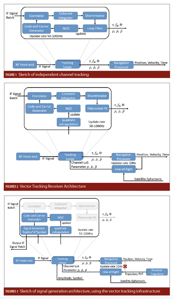 opportunity to manipulate the vector-tracking loop to generate replicas as needed to recreate signals that represent the receiver movements. In addition, the desired symbols and amplitudes must be provided to the tracking loops. Multiplying the replica signal with amplitude and symbol yields a new channel IF signal batch of samples. Adding up all channels produces an IF signal stream for a total or even multiple constellations. If required, additive white Gaussian noise (AWGN) can be added before the IF signal batch is written into the output stream. Ionospheric and tropospheric influences are simulated as the line-of-sight parameters are calculated using ionospheric and tropospheric models. The ST is able to track, generate, or regenerate tracked signals. A similar approach for regenerating tracked signals to upgrade existing receivers was presented by Humphreys et alia (Additional Resources).
We first present and explain the SR and the vector-tracking architecture. Thereafter, the modifications are described to convert a software receiver into a software transceiver, using the vector-tracking approach. The implementation as well as error sources are addressed, using the MuSNAT SR as foundation. We assess error sources and finally we compare the tracking and positioning performance of the ST generated signals with the theoretical limits and give examples for the current usage of the ST.
Software Receiver, Vector Tracking Architecture
Vector tracking is an old topic in the GNSS community and was first proposed in 1980 by Copps et alia. Since then, many papers, articles, and books have been published, describing and studying the topic in its full complexity and broadness with all its advantages and drawbacks (see Additional Resources). The references given are far from complete and can only be a starting point for interested readers.
To understand the necessary modifications for transforming a vector tracking-based SR into a signal generator (software transceiver, ST), a brief description of the conventional independent channel tracking architecture and the used vector tracking architecture follows.
All SRs have two main modules defining the processing workflow between the IF sample stream as receiver input and the receiver PVT information as receiver output: the signal processing unit with the tracking loops as its core, and the navigation processor. The signal processing unit, especially the tracking loops, process sample batches of the IF sample stream in sequential order and extract the pseudorange and pseudo range rate p for all tracked satellite signals. These parameters are passed to the navigation processor which then determines the receiver’s PVT.
In a conventional SR, separate and independent tracking loops track each satellite signal as a standalone signal. The signal processing is schematically shown in Figure 1. Each tracking loop consists of a correlator, integrator, discriminator, loop filter, NCO, as well as a code and carrier generator. The code and carrier generator create a replica of the received satellite signal. The replica generation parameters are controlled by the NCO. An early (E), prompt (P), and late (L) version of the generated replica signal is then correlated with the IF sample batch. The values for the integrated correlation signals are dumped and handed over to the discriminator. The discriminator evaluates the E, P, and L values for in-phase (I) and quadrature-phase (Q) and estimates the code time delay error as well as the carrier frequency error and the carrier phase error of the replica signal. Over the loop filter these estimated error values are used to update, i.e., speed up or slow down the NCO, so that the replica signal follows the satellite signal. A detailed description of the signal processing is provided in the Additional Resources. With the replica values, a good estimation of the satellite signal parameters (code delay, carrier Doppler, and carrier phase) can be determined. The satellite signal parameters are used to calculate the pseudorange and pseudorange-rate (Doppler) which are needed for the PVT determination in the navigation module. The update rate of the tracking loops is on the order of 50 to 1,000 hertz, whereas the navigation processor works with a common update rate on the order of 1 to 10 hertz. The loop filter with its bandwidth is used to smooth the high rate values for the NCO update. Therefore, the current smoothed output values of the loop filter are used by the navigation processor at the measurement epoch.
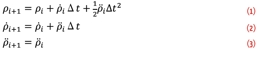
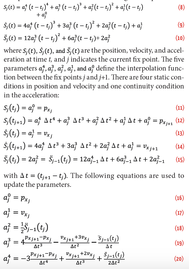
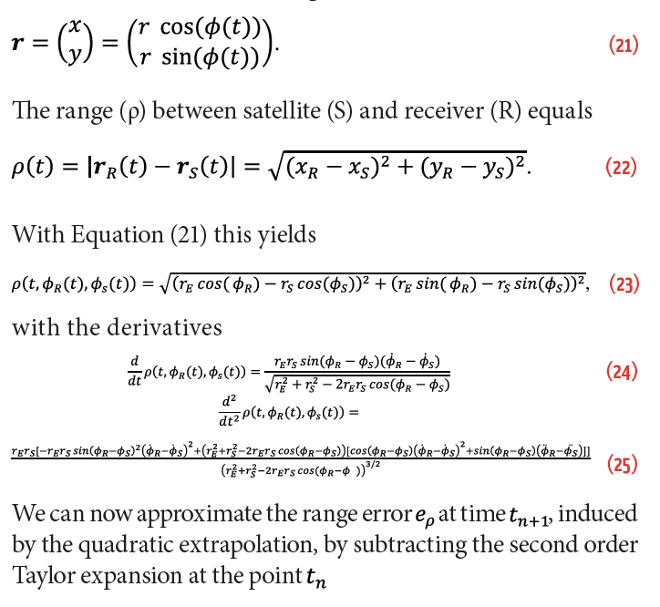
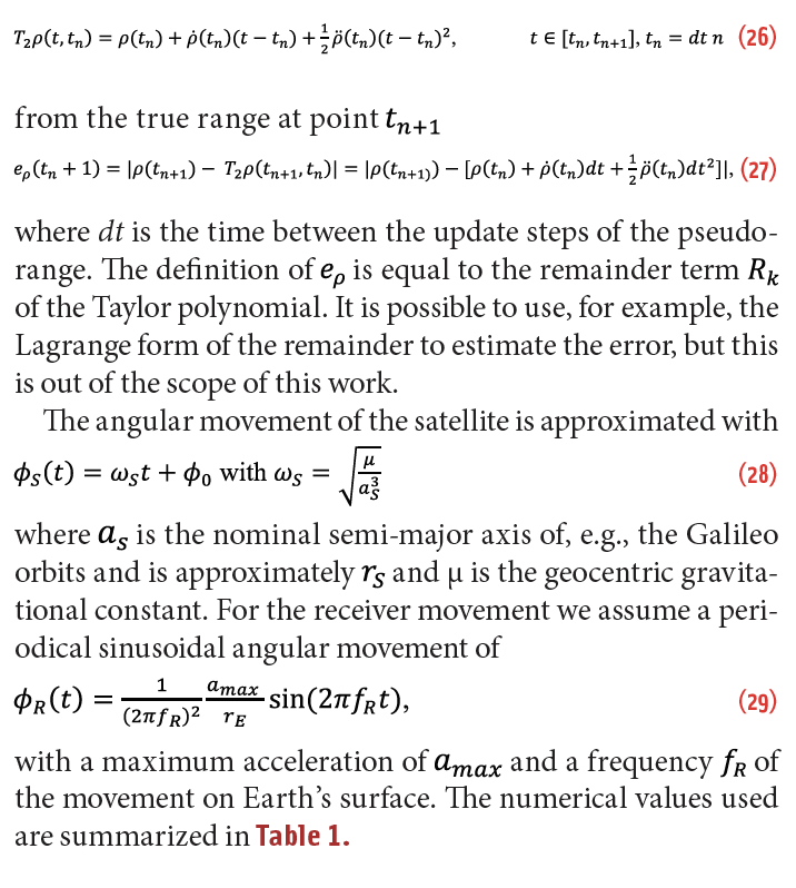
In a conventional SR all tracking loops work independently as mentioned above. This creates the drawback that the tracking loop can easily lose the satellite signal during short periods of signal blockage or signal fading. Even if the signal outage is short, the receiver must start with a reacquisition of the lost signal, which is time- and processing power-consuming. The basic idea of vector tracking is to support the single tracking loop with redundant information from the other tracking loops, so the single tracking loop is able to bridge periods of a weak signal or signal blockage. All satellite signal parameters are defined with respect to the PVT of receiver and satellite. Therefore, the PVT solution of the navigation processor represents the compressed information of the redundant tracking-loop outputs. The vector tracking task is to feedback this redundant information to each single tracking loop, or more precisely, to feedback the best estimation of it. This task can be realized in various forms, some more and some less complex. The more sophisticated approaches usually use some kind of extended Kalman filter (EKF) for PVT estimation (if this filter also includes inertial measurements, it is called a deep GNSS/IMU integration). The implementation used here is sketched in Figure 2, where the PVT algorithm is intentionally left unspecified. An additional module to determine the LOS parameters for all tracked satellites is needed. The satellite position is known from the ephemeris in the navigation message. The navigation module will update the LOS parameter with a rate of 10 hertz (100 ms). The operational update rate of the tracking loop, however, is around 1,000 hertz (1 ms). To overcome this lack of sampling points, a quadratic extrapolation of the LOS parameters is performed, assuming a constant acceleration until the next LOS update. The equations for the code extrapolation look like:
with ![]()
This extrapolation is obviously wrong in the long term but, as we will show later, for the short time span of 0.1 second the approximation works quite well for systems with moderate dynamics. These extrapolated LOS parameters are used to update the NCO in a hard reset fashion. This means that the replica signal changes during the 0.1 second in a smooth fashion, i.e., determined by Equations (1)–(3). After the update of the LOS parameters, however, a jump occurs in the range and range-rate domain of the replica signal parameters. The error of the extrapolation and the jumps of the replica signal are compensated in the pseudorange calculation, as the discriminator determines
![]()
For the carrier phase the Doppler values are integrated and reset at the reference epochs to match computed LOS phase values.
Due to the fact that the loop filter is no longer needed to determine the smoothed update values for the NCO, a new decimation filter is needed to provide smoothed pseudorange estimation values to the navigation processor. This can be a Kalman filter as in J.-H. Won et alia, but we use a polynomial fit method, where a vector of discriminator values is fitted with a polynomial function to determine the signal parameters at the measurement epoch (see again, T. Pany and B. Eissfeller).
Software Transceiver
An SR needs to mimic and create the satellite signals as well as possible to be able to track the signal hidden under the noise floor. So, all SRs are already signal generators. The only difference is that an SR reproduces an existing signal and is not creating a new one. To transform the SR vector tracking architecture into an actual signal generator, two main modifications (shown in Figure 3) must be applied.
First, one needs access to the created replica signal which consists of![]()
transceiver implementation following the concept described above. The implementation is based on the Multi-Sensor Navigation Analyzing Tool (MuSNAT) (Additional Resources).
Signal Generation
The MuSNAT SR processes IF sample batches of ~30 ms. This IF sample batch is divided into IF sample frames with a length of ~ 0.8 ms. The sample frames are processed in sequential order. In each processing step, the sample frame is distributed to all Master Channels. Each Master Channel processes one satellite signal and is composed of one or two tracking channels depending on whether the satellite signal has one (data) or two (data and pilot) components. All these channels process the sample frames successively. Due to this sequential workflow, we are able to allocate memory in the receiver with the same size as the IF sample batch and handover memory pointers to the tracking loops. In this way, all tracking loops can add their locally created satellite signal to this memory segment. When the IF sample batch processing is finished, the generated IF sample batch is processed in total. In this final processing step, AWGN can be added and output conversions can be performed. In the conversion step, the generated IF stream output format is set. Internally, the replica signals are stored as double-precision float values, to ensure minimal quantization errors in the signal addition process. For the saving process, the double values can be converted to the desired output format. In this work, either a real-valued 8bit or an I-Q-8bit conversion is used.
For the signal amplitude, we use predefined C/N0 values for each satellite in tracking. The amplitude parameter for each satellite s is defined as a relative amplitude. The reference satellite signal strength is 45 dB-Hz with an assigned reference amplitude of 1, weaker signals are assigned a corresponding smaller amplitude. The calculations were done with the equation
![]()
The standard deviation of the AWGN was calculated with:
![]()
where Aref=1 and C/N0ref = 45 dB-Hz, as the AWGN is adapted to the reference signal. The equations above were derived from M. Petovello and A. Joseph
![]()
where power![]() equals the sampling rate. SNR and BW denote the signal-to-noise ratio and the bandwidth. The amplitude value can also be used to implement a land mobile satellite (LMS) channel model (A. Lehner and A. Steingass) to simulate more realistic signal propagation conditions including multipath fading and blocking.
equals the sampling rate. SNR and BW denote the signal-to-noise ratio and the bandwidth. The amplitude value can also be used to implement a land mobile satellite (LMS) channel model (A. Lehner and A. Steingass) to simulate more realistic signal propagation conditions including multipath fading and blocking.
The last missing part for the signal generation represents the navigation symbol D. The navigation message has to be pre-produced and is stored in a receiver internal data base. D(t-τ) is selected for each sample frame according to the satellite transmitting time.
Here the SR usage provides the benefit that the data flow is already organized in a way that single frames refer to only one data symbol value.
User PVT Trajectory Feedback
For the user trajectory input we use a text file of the format shown in this example: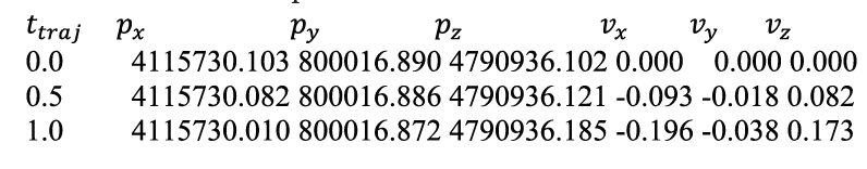
where traj is the trajectory time, Px, Py, and Pz represent the user position in the WGS 84 system in meters and represent the user velocity in the WGS 84 system in m/s. The trajectory points (2 hertz) need to be interpolated to the PVT update time steps (10 hertz). To do so, a fourth-degree spline interpolation approach was chosen. The fourth-degree spline interpolation is defined with the following three equations:
 The interpolations in the x, y, and z dimension are done independently from each other. The PVT solution also includes values for clock error and clock drift as well as accuracy estimations (mean radial spherical error, MRSE) for position and velocity. Clock error and clock drift are set to zero in a first step, position and velocity accuracy is set to 0.001 m and 0.001 m/s. These parameters can be defined in the trajectory input file and are set as needed. The interpolated PVT solution is handed over to the LOS module.
In this module, the LOS parameters are determined for all satellites in view and above a defined elevation angle. Therefore, the satellite position at the transmitting time is determined. Thereafter, the distance between satellite and receiver is calculated. In addition to Earth rotation and relativistic effects, ionospheric and tropospheric models are applied. The derivatives of the pseudorange are approximated by linear considerations.
In the next step, the LOS parameters are transferred to the tracking loops. Here a second extrapolation step is needed to adapt the sampling rate from the 10 hertz of the navigation process to the 1,000 hertz of the tracking loops. The quadratic extrapolation is already described above in the vector tracking section, see Equations (1)–(3). In the normal vector-tracking process, this approximation is acceptable because the error is compensated by the discriminator value. However, this approximation becomes an issue for the signal generation. The replica is created, following the extrapolated values, and a replica jump occurs at the edge of the last extrapolated point to the first point of the new extrapolation. These jumps could make it more difficult to track the generated signal, especially for the phase tracking. An assessment regarding this error follows in the next section.
Accuracy Assessment
Error model
The interpolation and extrapolation process is visualized in Figure 4 with a sinusoidal movement. Figure 4 is just for illustration purposes of the errors induced by the interpolation and extrapolation processes. To estimate the errors induced by the extrapolation process we use a very simple but representative user/satellite movement model. As the maximum values for
![]()
occur when the user movement and the satellite movement are in the same plane, we reduce the three-dimensional problem to the two-dimensional satellite orbit plane. The user movement is assumed to be only in this plane, on a spherical Earth with radius. The satellite orbit is also assumed to be circular with the radius. The 2-D movement model is sketched in Figure 5. In an Earth-centered-Earth-fixed (ECEF) frame, the receiver and satellite position can be calculated with
Error Simulation
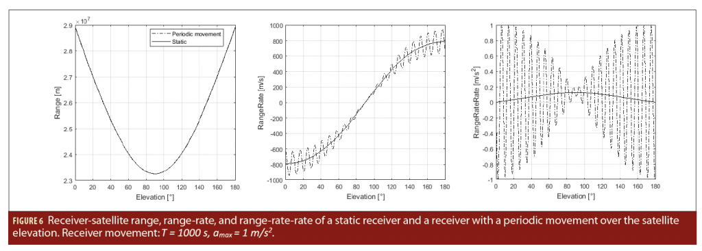
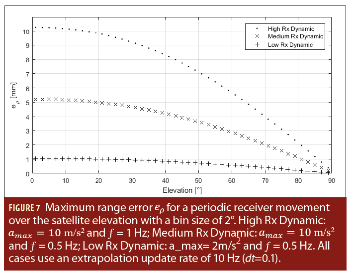
With Equations (23)–(25) we can calculate the range, range-rate, and range-rate-rate of a static or dynamic user. In Figure 6 the results for a static user and a user with a very long periodical movement are presented. The long periodical movement with a frequency of 0.001 hertz and a maximum acceleration of 1 m/s2 was chosen as it nicely illustrates the behavior over one total satellite cycle. The receiver movements are visible one-to-one in the range and its derivatives when the satellite has an elevation angle close to zero degrees. In contrast, the receiver movements vanish in the 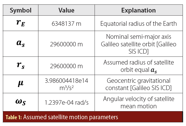 range values for an elevation angle of 90°. This was expected and is of no surprise but shows the correctness of our assumptions. In the next step we calculate the range error ep with Equation (27) and evaluate the maximum error for a specific satellite elevation for an extrapolation time dt=0.1 second. For the static receiver case there are only very small values and small variations for (see Figure 6), therefore, the extrapolation process is uncritical and is below 20 nm for all elevation angles. For a high dynamic receiver case we chose a maximum acceleration of and a movement frequency of 1 hertz. In this case the receiver changes its acceleration from +10 m/s2 to –10 m/s2 in 0.5 seconds. This is similar to an accelerating sports car whose driver later slams on the brakes. The maximum error over the satellite elevation is shown in Figure 7 (High Rx Dynamic). For the medium dynamic receiver case, we chose the values amax=2 m/s2 and f=0.5 hertz, Figure
 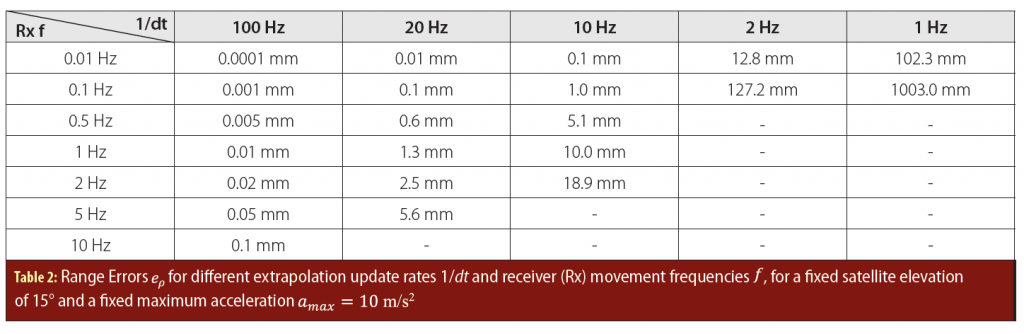 7 (Medium Rx Dynamic). A low dynamic receiver case is approximated with a maximum acceleration of (acceleration of a train) and a frequency of 0.5 hertz, Figure 7 (Low Rx Dynamic). Comparing the three different cases it is evident that the change in the maximum acceleration (medium versus low) has a similar impact on the total range error as a change in the dynamic frequency (high versus medium). As the approximation assumes a constant acceleration in the extrapolation time dt, it is clear that a fast change in the acceleration creates a significant influence on the range error. The second dominant parameter on the range error is of course the extrapolation time dt. In Table 2 the errors for different simulation parameters are listed for a fixed satellite elevation of 15° and a maximum acceleration of 10 m/s2. If we assume that a carrier phase error (jump) of 1% is tolerable, we end with the requirement <1.9 mm. Therefore, the extrapolation error is only acceptable for low and static receiver dynamics, using an extrapolation time of 0.1 second. If the update rate is increased to 100 hertz, even high receiver dynamics create only small extrapolation errors <<0.1 mm, again, see Table 2).
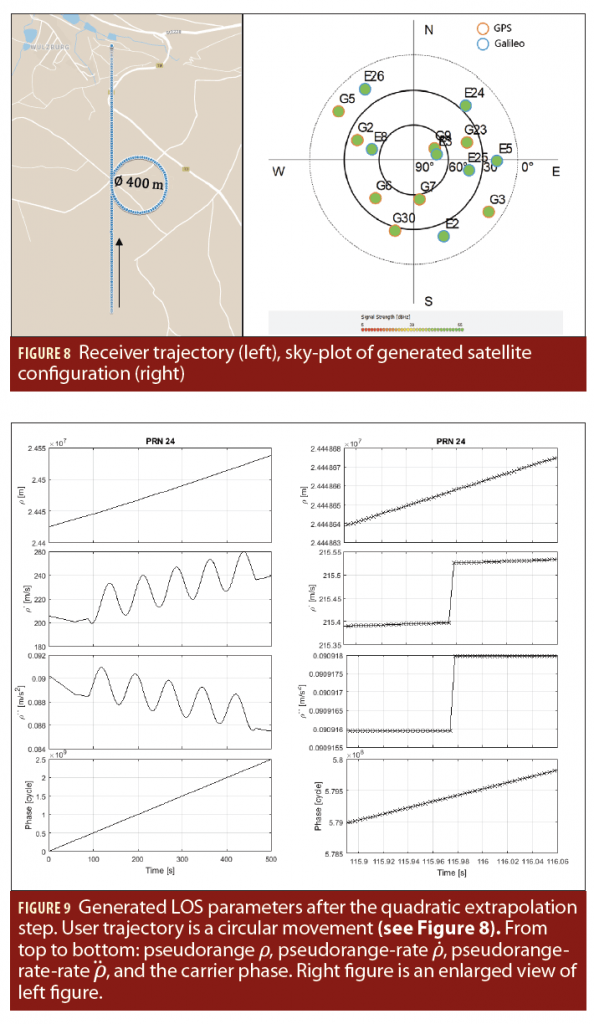
Results—Pseudorange Verification
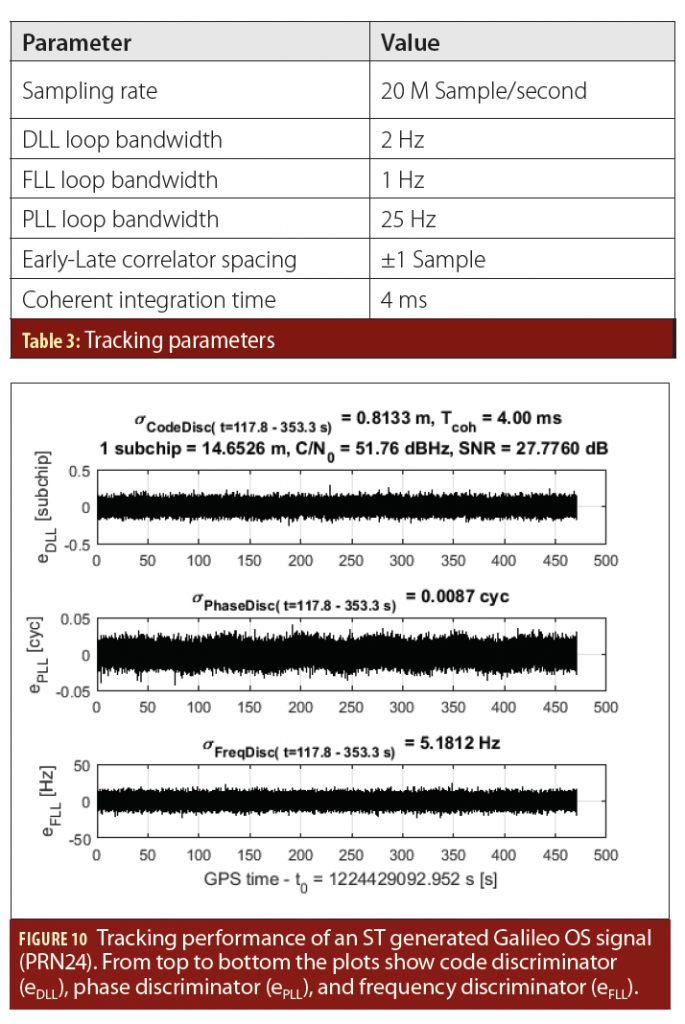
To verify the correct implementation and the consistent LOS parameter creation, the values for pseudorange, pseudorange-rate, pseudorange-rate-rate, and the carrier phase were plotted and evaluated using debug information for the respective build ST software module. The pre-defined receiver trajectory resembles a circle with a diameter of ~400 meters and the receiver velocity equals ~60 km/h, which results in a period of ~75 seconds and a frequency of ~0.013 hertz. The trajectory is plotted in Figure 8. The generated satellite configuration consists of eight GPS satellites and seven Galileo satellites, the sky-plot with all generated satellites is shown in Figure 8. The extrapolated LOS parameters of the Galileo satellite with PRN 24, are plotted in Figure 9. In the pseudorange plot and the phase only the satellite motion is visible as the pseudorange is governed by the satellite movement. In pseudorange-rate and pseudorange-rate-rate, however, the velocity and acceleration changes caused by the user movements are clearly visible. In the zoomed plot a constant behavior of and a linear behavior of is observed between the quadratic extrapolation jumps. For the pseudorange, no jump can be detected. These results match perfectly with the above described accuracy assessment. The expected range error for satellite PRN 24 (elevation 24°) with the described receiver movement is only on the order of ~12 μm.
Tracking and Positioning Performance
To check the quality of the generated signal, we compare in a first step the tracking performance of the generated signal with the theoretical value. The used tracking parameters are displayed in Table 3. The tracking results of the ST generated Galileo OS signal of PRN 24 are presented in Figure 10. The measured value for SNR was 27.776 dB and C/N0 = 51.76dB-Hz. According to these parameters, the theoretical values can be calculated as described by Thomas Pany (T. Pany in Additional Resources). The theoretical standard deviation of the code discriminator is. Comparing the measured standard deviation of small divergence of 2.1% can be observed and is similar to all tracked satellites. The results are very close to the theoretical minimum and proof a nearly perfect channel generation.
In a second step, the Single Point Position (SPP) of the tracking result was compared with the initially defined (“real”) user trajectory. Therefore, the seven Galileo satellites were used for the SPP solution. In Figure 11, the error δ of the SPP solution to the “real” trajectory is plotted in the local east-north-up coordinate frame. The mean position error and the standard deviation error of the SPP position in the east, north, and vertical directions are given in Table 4. The theoretical values are calculated with
![]()
where DOP is the Dilution Of Precision value in the corresponding direction and is the pseudorange standard deviation with a theoretical value of 0.090 m. A comparison of the values is given in Table 4. As indicated in Table 4, a gap exists between the theory and the measured noise values of 2–4 decimeters. The reason for the difference is not clarified yet and is under investigation, however, the very small mean position errors prove a bias-free position generation.
Areas of Application
The MuSNAT signal generator was already used to implement and verify Navigation Message Authentication (NMA) (see Additional Resources) foreseen for Galileo Open Service (OS) signals. In this activity, real Galileo satellite signals were recorded and processed with th
e MuSNAT to extract the symbol-stream (navigation message) and satellite ephemeris for each satellite in sight. In the second step, the spare bits in the Galileo E1B INAV navigation message are replaced with the OSNMA authentication bits. Thereafter, the symbol stream, the satellite ephemeris, and the desired C/N0 values for the tracked satellites were read into the GNSS-Transceiver to generate the IF sample-stream file. For analysis, the IF sample file was again processed by the MuSNAT-Transceiver to extract the bits and verify the authentication. The detailed analysis of the NMA is presented by Maier et alia. In the same work, Maier et alia used the MuSNAT signal generator to study the influence of secure code estimation and replay (SCER) attacks (again, see Additional Resources) on a software receiver. In contrast to the NMA test, these tests would not be possible with a COTS signal generator system, due to the need for modifying the generated signal on a deeper level.
Conclusion and Outlook
In this work, it was shown that the conversion of a software receiver into a software transceiver using the vector-tracking approach is feasible and quite easy to realize. The basic concept was presented with an accuracy assessment on the error sources. The implementation of the concept using the MuSNAT software receiver was explained. The quality of the generated signals was compared with the theoretical lower limits. It was shown that the satellite channel could be generated very accurately.
As shown in the accuracy assessment section, the extrapolation range error varies over a wide range, depending on the satellite elevation, the maximum acceleration, the acceleration change rate, and the extrapolation time. The range error is below 1 mm even for high receiver dynamics if an update rate of 100 hertz is chosen. For an update rate of 10 hertz only static and slow receiver movements can be generated with sufficient accuracy. As the current generator settings use an update rate of ~10 hertz, it is planned to increase the update rate and study the possibility of replacing the quadratic extrapolation step with an interpolation, very similar to the trajectory interpolation. To do so, not only the current LOS parameters but also the future LOS parameters need to be passed to the tracking loop. These updates will allow us to create continuous and consistent satellite signals for all possible receiver dynamics. Additionally, the implementation of LMS channel models is planned to increase the realism of the signal generation.
Acknowledgments
This work is funded by the German Federal Ministry for Economic Affairs and Energy on the basis of a decision by the German Bundestag. It is administrated by the German Aerospace Center in Bonn, Germany, (FKZ: 50 NA 1703)
Additional Resources
(1) Copps, E. M., G. J. Geier, W. C. Fidler, and P. A. Grundy, “Optimal Processing of GPS Signals,” NAVIGATION, Volume: 27, Issue: 3, pp. 171-182, 1980.
(2) Fernández-Hernández, I., V. Rijmen, G. Seco-Granados, J. Simon, I. Rodríguez, and J. D. Calle, “A Navigation Message Authentication Proposal for the Galileo Open Service,” NAVIGATION, Volume: 63, Issue: 1, pp. 85-102, 2016.
(3) Galileo SIS ICD, “European GNSS (Galileo) Open Service Signal-
In-Space Interface Control Document,” OS SIS ICD, Issue 1.3, 2016.
(4) Humphreys, T., B. Jahshan, and L. Brent, “The GPS Assimilator: A Method for Upgrading Existing GPS User Equipment to Improve Accuracy, Robustness, and Resistance to Spoofing,” Proceedings of the 2010 ION Conference, Portland, 2010.
(5) Humphreys, T. E., “Detection Strategy for Cryptographic GNSS Anti-Spoofing,” IEEE Transactions on Aerospace and Electronic Systems, Volume: 49, Issue: 2, pp. 1073-1090, 2013.
(6) Institute of Space Technology and Space Applications (ISTA), “MuSNAT,” URL: https://www.unibw.de/lrt9/lrt-9.2/software-packages/musnat/view, September 2018.
(7) Kerns, A. J., K. D. Wesson, and T. E. Humphreys, “A Blueprint for Civil GPS Navigation Message Authentication,” Proceedings of the IEEE/ION 2014 Position, Location and Navigation Symposium (PLANS), pp. 262-269), 2014.
(8) Lehner, A. and A. Steingass, “A Novel Channel Model for Land Mobile Satellite Navigation,” Proceedings of ION GNSS 2005, 2005.
(9) Maier, D., K. Frankl, R. Blum, B. Eissfeller, and T. Pany, “Preliminary Assessment on the Vulnerability of NMA-based Galileo Signals for a Special Class of Record & Replay Spoofing Attacks,” Proceedings of IEEE/ION PLANS 2018, Monterey, CA, pp. 63-71, April 2018.
(10) Pany, T. and E. Bernd, “Use of a Vector Delay Lock Loop Receiver for GNSS Signal Power Analysis in Bad Signal Conditions,” Proceedings of the 2006 IEEE/ION Position, Location, And Navigation Symposium (PLANS), 2006.
(11) Pany, T., Navigation Signal Processing for GNSS Software Receiver, Artech House, 2010.
(12) Parkinson, B. W., P. Enge, P. Axelrad, and J. J. Spilker,Jr., eds., Global Positioning System: Theory and Applications, Volume II, American Institute of Aeronautics and Astronautics, 1996.
(13) Petovello, M.G. and C. T. Curran, “18. Simulators and Test Equipment,” Springer Handbook of Global Navigation Satellite Systems, Springer, 2017.
(14) Petevello, M., M. Lashley, and D. M. Bevly, “What are Vector Tracking Loops, and What are their Benefits and Drawbacks?,” Inside GNSS, May/June, 2009.
(15) Petovello, M. and A. Joseph, “Measuring GNSS Signal Strength,” Inside GNSS, November/December, 2010.
(16) Psiaki, M. L. and T. E. Humphreys, “GNSS Spoofing and Detection,” Proceedings of the IEEE, Volume: 104, Issue: 6, pp. 1258-1270, 2016.
(17) Stöber, C., M. Anghileri, A. Sicramaz Ayaz, D. Dötterböck, I. Krämer, V. Kropp, D. Sanromà Güixens, J.-H. Won, B. Eissfeller, and T. Pany, “ipexSR: A Real-Time Multi-Frequency Software GNSS Receiver,” Proceedings of the IEEE 52nd International Symposium ELMAR, 2010
(18) Wesson, K. D., M. P. Rothlisberger, and T. E. Humphreys, “A Proposed Navigation Message Authentication Implementation for Civil GPS Anti-Spoofing,” Proceedings of the Radionavigation Laboratory Conference, 2011.
(19) Won, J.-H., D. Dominik, and E. Bernd, “Performance Comparison of Different Forms of Kalman Filter Approaches for a Vector-Based GNSS Signal Tracking Loop,” NAVIGATION, Volume: 57, Issue: 3, pp. 185-199, 2010.
(20) Won, J.-H. and T. Pany, eds., “14. Signal Processing,” Springer Handbook of Global Navigation Satellite Systems, Springer, 2017.


