In February 2011, Russia launched the first satellite of the GLONASS-K1 series, i.e., SVN (space vehicle number) 801 (R26), which in addition to the legacy frequency division multiple access (FDMA) signals, for the first time was enabled to transmit code division multiple access (CDMA) signals on the GLONASS L3 frequency (1202.025 MHz). Later in 2014, the GLONASS program added SVNs 802 (R17) of series K1 and 755 (R21) of series M, and in 2016, SVN 751 of series M, with the capability of transmitting CDMA L3 signals to the constellation.
In February 2011, Russia launched the first satellite of the GLONASS-K1 series, i.e., SVN (space vehicle number) 801 (R26), which in addition to the legacy frequency division multiple access (FDMA) signals, for the first time was enabled to transmit code division multiple access (CDMA) signals on the GLONASS L3 frequency (1202.025 MHz). Later in 2014, the GLONASS program added SVNs 802 (R17) of series K1 and 755 (R21) of series M, and in 2016, SVN 751 of series M, with the capability of transmitting CDMA L3 signals to the constellation.
The GLONASS FDMA double-differenced (DD) ambiguity resolution is known to be hampered by the inherent inter-frequency biases. Several calibration procedures have been proposed to deal with this impediment. With GLONASS-CDMA however, the standard methods of integer ambiguity resolution can be applied to resolve the integer DD ambiguities. The goal of this article is to provide a first assessment of this L3 ambiguity resolution performance.
Measurement Setup
Our analysis is based on the GLONASS L3 data of the satellite pair R21-R26, collected by two multi-frequency GPS/GLONASS receivers on an eight-meter baseline at Curtin University, Perth, Australia (Figure 1). We also compare these results with their GPS L5 counterparts for the satellite pair G10-G26. The rationale behind making this comparison is that both these modern signals have close frequencies (see Table 1) and the same BPSK(10) modulation.
Figure 2 shows their observed carrier-to-noise densities (C/N0).As their C/N0 graphs show a similar signature, their signals are expected to have similar noise characteristics. Figure 1 also shows the skyplot of the mentioned satellite pairs at Perth. For both the GLONASS and the GPS satellites, we used the broadcast ephemeris data. Table 2 provides further information on the data-set that we used.
Model of Observations
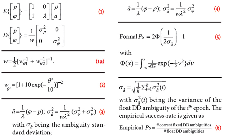
Because our analysis is based on satellite pairs, we first formulate the two-satellite observational model. With the expectation E{.} and dispersion D{.}, the corresponding double-differenced (DD) system of observation equations reads
Equation (1) (see inset photo, above right, for all equations)
in which p and φ are the DD code and phase observable, respectively, ρ the DD receiver-satellite range and a the DD integer ambiguity in cycles. The ambiguity a is linked to the DD phase observable through the signal wavelength λ. With the elevation-dependent weighting function wθs (s = 1, 2) for the sth satellite with elevation angle θs, respectively, the final weight becomes
Equation (1a)
Here wθs is taken as
Equation (2)
where θs is in degrees. The zenith-referenced standard deviations of the undifferenced code and phase observables are denoted as σp and σφ. In our analysis we considered two different models. These are arranged in ascending order of strength as:
1. Geometry-free model (GFr): This is the model as formulated in (1). As it is parametrized in ρ, it is free from the receiver-satellite geometry. The single-epoch DD ambiguity is then estimated as
Equation (3)
2. Geometry-fixed model (GFi): In this model, the information on receiver position, from e.g. surveying, and satellite position, from navigation file, is available and thus ρ is assumed known. The single-epoch DD ambiguity is then estimated as
Equation (4)
Note that although the observations of only two satellites are used, both the geometry-free and geometry-fixed models are instantaneously solvable, i.e., based on data of only a single epoch. See the article by P. J. G. Teunissen (1997) listed in the Additional Resources section near the end of this article for a more detailed discussion of these models.
Ambiguity Resolution
The data used for our L3 and L5 ambiguity resolution performance analysis were one hertz sampled on DOY 21 of 2016 over the time period UTC [07:16:59-09:13:38]. As the observations of a satellite pair and a receiver pair result in only one unknown DD ambiguity, simple integer rounding can be used for integer ambiguity resolution. We denote the float ambiguity by â, the fixed (integer rounded) ambiguity by ă, and the reference ambiguity by a. The reference DD ambiguity a is computed based on the multi-epoch solution of the geometry-fixed model.
In Figure 3, the time series of â − a and ă − a are shown for the receiver pair CUT3-CUCC, for both the GLONASS satellite pair R21-R26 (left column) and the GPS satellite pair G10-G26 (right column).
While the geometry-fixed results of the two signals are comparable, the GPS L5 geometry-free ambiguity resolution outperforms that of the GLONASS L3, which can be explained by means of the satellites’ elevations: the higher the elevation, the lower the noise level, thus the better the ambiguity resolution performance (cf. 2, 3 and 4).
The bottom set of graphs in Figure 3 also illustrates the elevation time series of the chosen satellite pair (in blue) in addition to the geometry-fixed DD ambiguities. Here we can see that the elevations of the GPS satellite pair is higher than those of the GLONASS satellite pair. Also, the low elevation of R26 at the end of the period and the low elevation of G10 at the beginning of the period describe the larger fluctuations of, respectively, the GLONASS DD ambiguities and the GPS DD ambiguities at those time instants.
For both the geometry-free and the geometry-fixed scenario, we computed the formal and empirical ambiguity success-rates, defined as the probability of correct integer estimation. The formal ambiguity success-rate can be computed, as discussed in the article by P. J. G. Teunissen, (1998) cited in Additional Resources, as
Equation (5)
being the standard normal probability density function (PDF).
For the computation of the formal success-rate, the ambiguity standard deviation was taken as the square-root of an average of the formal variances, i.e., as
Equation (6)
Table 3 lists the empirical and formal success-rates for both GLONASS and GPS corresponding with Figure 3. Based on these results, the empirical values are consistent with their formal counterparts. Moreover, as the model gets stronger from one-epoch geometry-free to geometry-fixed, the ambiguity resolution success-rates experience a significant improvement. In case of the one-epoch geometry-free model, σâ is governed by the code precision σp. Including the observations of k epochs, the corresponding σâ of k-epoch geometry-free model is improved by almost √ k
times.
Switching from geometry-free to geometry-fixed model, σâ is then governed by the phase precision σφ which is much better than the code precision. For the geometry-free model to achieve a success-rate of more than 0.999, 40 epochs of observation in the case of GLONASS L3 and 10 epochs in the case of GPS L5 are required.
To further confirm the consistency between the data and models, we compare, for both the geometry-free and the geometry-fixed model, the formal PDF with the histogram of the estimated DD ambiguity. Normalizing the estimated DD ambiguity by means of the elevation weighting function results in a new quantity, i.e., √ w (â – a) which, assuming the data to be normally distributed, has a central normal distribution with the standard deviation of √ w σâ. Depending on whether the underlying model is geometry-free or geometry-fixed, the value of √ w σâ can be obtained from (3) or (4), respectively.
Figure 4 displays the histograms of the normalized DD ambiguity √ w (â – a), for geometry-free and geometry-fixed model. The corresponding formal distribution is also shown by the red curve. It demonstrates the consistency between the empirical and formal distributions.
Conclusion
We have presented a first assessment of GLONASS CDMA L3 double-differenced integer ambiguity resolution.
For our analyses, we made use of the GLONASS L3 signal transmitted by the satellite pair R21-R26 and of the GPS L5 signal from the satellite pair G10-G26. The carrier-to-noise densities of both signals were shown to have similar signatures.
The integer ambiguity resolution performance in the framework of geometry-free and geometry-fixed observational model was demonstrated. As the model gets stronger from geometry-free to geometry-fixed model, the ambiguity resolution improves significantly.
Our empirical results (in the form of success-rates and normalized ambiguity PDF) showed a good agreement with their formal counterparts, thereby showing the consistency between data and models. The ambiguity resolution of GPS L5 was better than that of the GLONASS L3, which was attributed to the higher elevation of the GPS satellites w.r.t the GLONASS satellites during the considered period.
Additional Resources
[1] Euler, H. J., and C. C. Goad, “On Optimal Filtering of GPS Dual Frequency Observations without Using Orbit Information,” Bulletin Geodesique 65(2):130-143, 1991
[2] Global Positioning Systems Directorate, NAVSTAR GPS space segment/navigation user segment Interface Specification, Revision F (IS-GPS-200H:24-Sep-2013)
[3] Hofmann-Wellenhof, B., and H. Lichtenegger and J. Collins, Global Positioning System: Theory and Practice, Springer Science & Business Media, 2013
[4] Information and Analytisis Center for Positioning, Navigation, and Timing, GLONASS constellation status, available here, accessed February 2, 2016
[5] Leick, A., GPS Satellite Surveying, John Wiley and Sons, 2003
[6] Oleynik, E., “GLONASS Status and Modernization,” United Nations/Latvia Workshop on the Applications of Global Navigation Satellite Systems, Riga, Latvia, 2012
[7] Reussner, N., and L. Wanninger, GLONASS Interfrequency Biases and Their Rffects on RTK and PPP Carrier-Phase Ambiguity Resolution,” Proceedings of ION GNSS 2011, Institute of Navigation, pp. 712-716, 2011
[8] Takac, F., “GLONASS Inter-Frequency Biases and Ambiguity Resolution," Inside GNSS, 4(2):24-28, 2009
[9] Teunissen, P. J. G., (1997) “A Canonical Theory for Short GPS baselines. Part I: The Baseline Precision,” Journal of Geodesy, 71(6):320-336, 1997
[10] Teunissen, P. J. G.,(1998) Success probability of integer GPS ambiguity rounding and bootstrapping. Journal of Geodesy, 72(10):606-612, 1998
[11] Thoelert, S., and S. Erker, J. Furthner, M. Meurer, G. X. Gao, L. Heng, Walter, and P. Enge, “First Signal in Space Analysis of GLONASS K-1,” Proceedings of ION ITM 2011, pp. 3076-3082, 2011
[12] Urlichich, Y., and V. Subbotin, G. Stupak, V. Dvorkin, A Povaliaev and S. Karutin,(2010) GLONASS Developing Strategy,” Proceedings of the 23rd ION ITM 2010, Institute of Navigation, pp. 1566-1571, 2010
[13] Urlichich, Y., and V. Subbotin, G. Stupak, V. Dvorkin, A Povaliaev and S. Karutin, (2011), “A New Data Processing Strategy for Combined GPS/GLONASS Carrier Phase–Based Positioning,” Proceedings of the ION GNSS 2011, Institute of Navigation, pp. 3125-3128, 2011
[14] Wanninger, L., “Carrier-Phase Inter-Frequency Biases of GLONASS Receivers,” Journal of Geodesy, 86(2):139-148, 2009
[15] Yamada, Y., and T. Takasu, N. Kubo, and A. Yasuda, “Evaluation and Calibration of Receiver Inter-Channel Biases for RTK-GPS/GLONASS,” Proceedings of ION GNSS 2010, Institute of Navigation, pp. 1580–1587, 2010


