End Game for Urban GNSS: Google’s Use of 3D Building Models

When GPS/GNSS was first developed in the 1970s, it was premised on line-of-sight signals with expected civilian accuracy of tens of meters. Almost immediately, commercial industry pioneers began to use GPS outside its intended design envelope. Almost all the accuracy, signal processing, and use-case limitations were solved: differential GNSS, carrier phase positioning, assisted GNSS, high sensitivity, and even GNSS in space.

One great unsolved problem is inaccuracy in cities.

GNSS constructively places you on the wrong side of street or the wrong city block, in a situation where line-of-sight (LOS) signals are blocked, because the receiver tracks the non-line-of-sight (NLOS) signals reflected off buildings, and the entire system assumes line-of-sight time-of-flight. Now Google has deployed a system that solves this problem.

Using Google’s vast database of 3D building models, the asymmetric NLOS propagations are modeled so that the NLOS pseudorange errors can be corrected, leading to 50 to 90% reduction in wrong-side-of-street (WSS) occurrences from GNSS in phones.

The Problem

NLOS reflections in cities create one of the last great unsolved GNSS problems. Let’s take a walk through the last 40 years of GNSS to see why. The GPS system was first built in the 1970s, and the concept was, and remains, that the receiver measures its distance from the satellites from the time-of-flight of the signal.

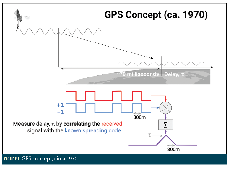
Let’s take a brief look at how the receiver measures the time delay, because this is going to be very important to us when we get to the L5 signal. The signal from the satellite is a carrier wave, modulated by a square wave spreading code. As shown in Figure 1, the receiver strips off the carrier, leaving the spreading code (shown in red), and correlates with its own copy of the same code (blue). Red combined with blue = purple, and we get the triangular correlation response.

The key feature of the L1 civilian code is that the length of the spreading code bits is 300m. Thus the correlation response triangle has a base of 600m.

Back in the 70s the anticipated accuracy of the system, if you used the 10x faster military P code, was “order of 10m” [MZ 78].

By the 80s the situation had already changed radically. Firstly there was much better signal processing, such as what became known as “narrow correlators.” So long as you were under open sky, then the 300m spreading code proved less of an accuracy problem than anticipated. Then came differential GPS (DGPS). By the end of the 80s civilian DGPS accuracy was approximately one meter.

Looking at the carrier wave itself, with a phase-locked-loop the receiver measures carrier-phase to a fraction of the wavelength. Combined with DGPS and phase ambiguity resolution, real-time centimeter accuracy became standard for surveyors in the 90s.

With the FCC E911 mandate, attention turned to making GPS work in a cell phone. It’s easy to forget that in 1999 GPS was considered a long shot to provide location technology in phones, and the initial E911 implementations were done with cellular-signal time-of-arrival. GPS was too slow and too power-hungry. This spurred Assisted GPS development, resulting in 1-second time-to-fix and +30dB (1,000x more) sensitivity. This is now standard in all smartphones, and none of us think twice about the magic of our blue dot showing up almost instantly whenever we open Google Maps.

So by this century GPS is found in use, with high speed, high sensitivity, and great accuracy, anywhere where you have a view of the open sky.

In the last 10 years, spoofing and jamming have emerged as real threats to GNSS. They remain threats, however, there is a known solution to this problem, if you have the means to implement it. This is to have a phased-array antenna, and construct beams for each channel only in the direction of the satellite of interest. This is, of course, quite difficult to realize in practice, but the point is that it is at least possible. Contrast this with the problem that we face in cities:

Suppose you’re tracking a few satellites; and every one of them is non-line-of-sight; and the LOS direct signals are all completely blocked. What you’re tracking are the reflections. How do you solve for position? Until recently this was an unsolved problem.

This is our great unsolved problem. Until the deployment of the 3DMA solution presented here, the GNSS in any smartphone would tend to put you on the WSS if not the wrong city block in this scenario.

Intellectually, this is a great challenging problem. But what about commercially—is this important? The answer is a resounding Yes!

Based on our own tests, and knowing the number of phones in use. We estimate that there are over 1 billion fixes per day on the WSS or worse. This destroys pedestrian GNSS navigation and ride-share-pickups. This is the problem we set out to solve.

Approaches to Date

The oldest and best researched solution to reflected signals is to depend on inertial navigation systems (INS). INS-GNSS integration is built into all smartphones and will engage automatically when you are driving and the phone is mounted in an inertially stable way (like on the dashboard). The INS integration will solve the urban canyon problem when you first drive into a city. But, it will do nothing for you as you start up your GNSS while already in the city, or if you drive for too long in the city especially with lots of stops.

The next best researched solution is “shadow matching.” You can understand this easily by analogy with the Sun. Consider the Sun is casting shadows from some buildings. If someone told you they were in the shadow, you’d know immediately the region they must be in. Correspondingly, if they were in the sunlight.

Similarly, you can measure the signal strength (or carrier to noise ratio) of GNSS signals, and make similar inferences. Intersect such regions for many satellites, and you can work out your location—in principle.

However, in practice GNSS signals strengths in phones are all over the place. How do you draw the line between strong and weak?

We can bring a little bit of order by doing analysis with known ground truth and computing LOS or NLOS for each satellite at each time, and coloring LOS blue and NLOS brown. In Figure 2, blue is generally on the top, and brown on the bottom. However, at any moment you will see LOS signals that are weaker than almost all the NLOS signals. And conversely, NLOS signals that are strong.

Nonetheless, there is useful statistical information here, and there is a lot of research that shows useful results in small scale experiments. See approximately 70 papers by Paul Groves, UCL, on this topic.

Next there is a similar approach, matching measured pseudorange to predicted values across a grid. At each grid point you calculate what you expect to measure taking the NLOS reflections into account. The challenge here has been that the ray-tracing was an overwhelming computational challenge. More on ray-tracing below.

In summary:

• INS integration works when driving into a city.

• For pedestrians, or cars starting up in a city, there are some promising ideas: shadow matching, and pseudorange matching.

Both show promise on small trials (typical research=1 to 10 data traces in a single city). But also significant challenges (e.g., C/N0 variations, trees, computation time, differences in city characteristics, widespread availability and accuracy of 3D models). And nothing was deployed at scale before 2020.

A Complete Solution for a Limited Case

The reflected path-length errors are different depending on where you are standing. This creates the following chicken-egg problem:

• If we knew our position, and the 3D building models, then we could compute the reflection errors, remove them, and then accurately compute our position.

• But we don’t know our position!

The problem is that the NLOS errors are a function of our unknown position.

The trick is to use this problem as the solution, by writing a math function to express the reflection errors uniquely in terms of the unknown x, y, z, and then solve the resultant equation for x, y, z. We can do this if we make the assumption that we know the reflecting surfaces. This results in a modification to the classic GNSS navigation equations that fully account for the reflections. A full description of the mathematics will appear in a separate publication.

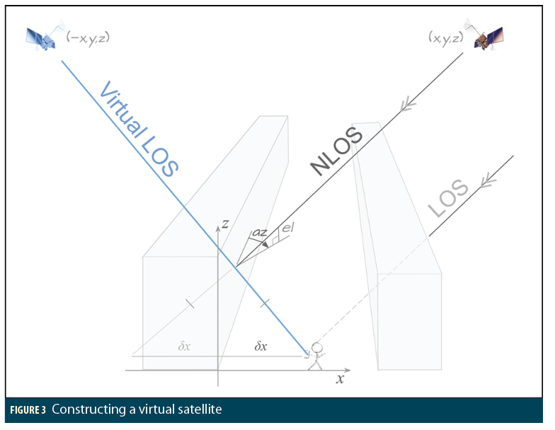
An equivalent approach is to construct a virtual satellite by reflecting the satellite position about the reflecting plane, and then solving in the normal way, as-if LOS. This idea has been investigated for 2D WiFi positioning [G 16], and direct GNSS positioning [NG 16]. The beauty of this approach is that, as long as we know the reflecting surfaces, we can construct the virtual satellite position. Thus we traverse the chicken-egg problem (Figure 3).

However, there is a subtlety here that is worth further discussion: The normal GPS solution requires that you rotate the reference frame to account for Earth rotation between time of transmission (ttx), and time of reception (trx). If you fail to do this you get errors of the order of 30m, because that’s about how much the Earth rotates in the time-of-flight of the GPS signal. (In 70 milliseconds, a point on Earth rotates 32m at the equator, 24m at 40° latitude, e.g. New York.)

So, if you are computing the reflected position of the satellite, do you use the reflecting plane location at a) ttx, b) trx, c) the average, or d) it makes no difference?

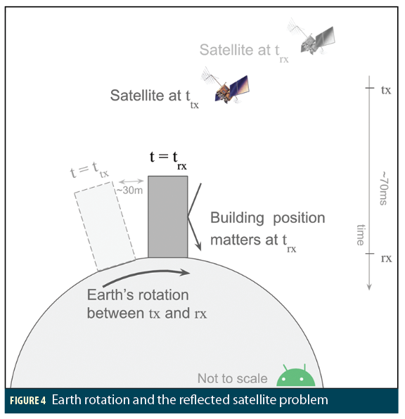
The answer is: b) you must use the reflecting plane position at trx. Let’s see why (Figure 4):

The satellite position matters at ttx. Then, while the signal travels to Earth, the Earth rotates, and the signal arrives at trx. And so the building position matters at trx (the location of the building at ttx is irrelevant).

Even this subtlety has a subtlety. Strictly speaking, we should use the time of the reflection, which is ~0.2 microseconds before trx at the receiver (for typical city geometries). But the Earth rotates less than 0.1mm in this time, and so for our purposes we can safely use trx.

In summary for this section: if we knew the reflecting planes, then using either an adjustment to the classic nav equations, or the reflected satellite positions, we can solve this problem—even if all signals are NLOS.

However, the typical case is much more complex, in 3 ways:

• There are many different reflectors for each signal. As you can see from the ray tracing figure below.

• The reflecting surfaces are not mirrors but scatterers, and sometimes diffractors.

These two are not fatal—and provide fertile ground for future research. But the last issue is the killer:

• We frequently don’t know the reflecting surfaces, or even which street we are on.This prevents us from using the neat solution just described; and we are forced to take a more general approach.

Google-scale Approach

To start, you must have 3D models. Luckily we have these, in abundance.

Google has deployed 3DMA-GNSS in Android phones for almost 4,000 cities, covering major cities in North America and Europe, Japan, Taiwan, Brazil, Argentina, Australia, New Zealand, and South Africa. Tests are ongoing in other places.

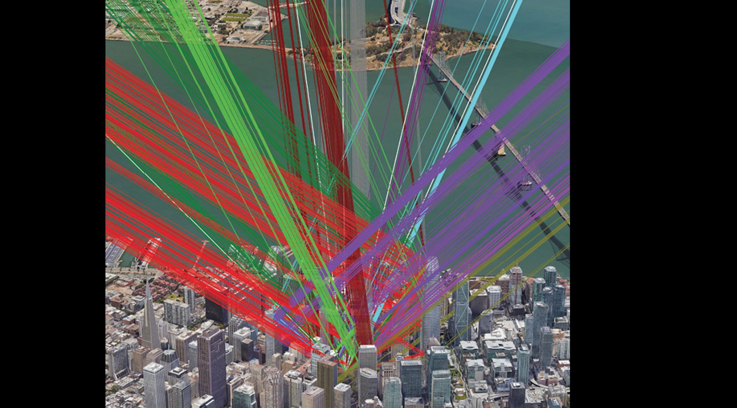
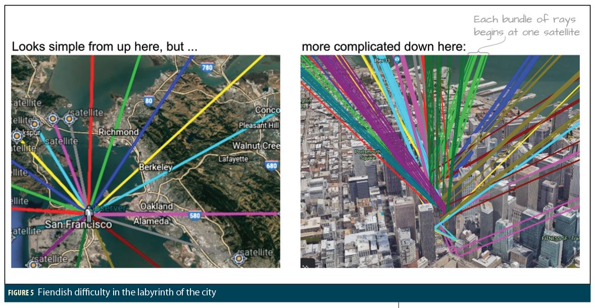
Once you have accurate 3D models, you can do ray tracing (Figure 5). These two pictures are the same, but the left one looks simple, while the right one, which is just a zoom-in of the left, shows the fiendish difficulty awaiting us in the labyrinth of the city.

Generally we try to avoid O(N2) complexity in programming (like a nested loop). The ray tracing problem for an NxN grid is O(N2P3), where P is the number of rays. With multiple reflecting surfaces, scattering and diffraction, P can get very large, which means it is more than your phone can handle, unless you do something smart.

In our implementation we use all of the above: 3D buildings, ray tracing, raw measurements, the best of the published research, plus a Bayesian approach to deal with variations in measurements. Finally, and most importantly, machine learning, discussed next.

Machine Learning (ML)

ML can work to compute GNSS locations. I won’t go into detail, but if you can see the way in which ML works, then that’s enough. Also, where I use the standard terminology of ML it is italicized, so you can pick up some vocabulary as you read this section.

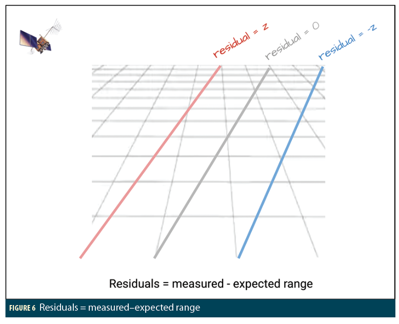
First, it’s important to think about GNSS in the right way. The idea of imaginary spheres of range around each satellite is not useful. Instead, think about a grid of possible locations in the approximate region that we know we are. Then consider the residuals, that is, the measured minus expected range at each grid point. Where the measured and expected ranges match, we get a line-of-position for residual=0.

If you think of points closer to the satellite then the expected range is smaller, so the residual gets bigger, and conversely, in the opposite direction it gets smaller (Figure 6).

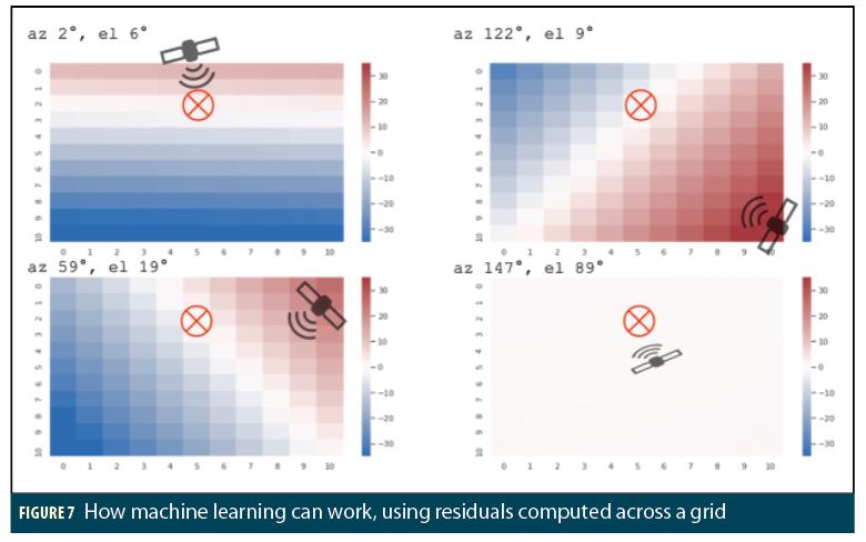
Here is a toy example: something we know how to do, just to show how ML can work. We have measurements from 4 satellites, collected in an area with open sky and no obstructions.

Figure 7 shows the four grids, one for each satellite, and the residuals for each satellite, color coded where more red is more positive, more blue is more negative. And white is where the residuals=0.

As you can see, the correct position lies at the red . For this example we removed the clock bias in advance to make it easy for us humans to understand. So you would expect that the position solution lies on the lines of position where residual=0. But realize that what we just did was find the intersection of planes. The residuals form planes across the grid. And the position solution is the intersection of the planes. This holds true regardless of the clock bias.

Now, how do we teach a machine to learn that it should seek out the intersection of planes?

We build a neural network (NN) connecting all our inputs (residuals) to the desired output (position). Each neuron is a linear combination of its inputs, (e.g. subtraction of residuals from different satellites) followed by an activation function (a non-linear operation, that can approximate any function, e.g. absolute value).

The network (Figure 8) learns which combinations correspond to the known ground truth in millions of training examples. For our toy example you can see how this network could learn to find where the residuals all match, which is the intersection of the planes from the previous image.

This is a picture of the actual neural network built for our toy example. Each box represents many neurons connected together. After training the network with millions of examples, each consisting of residuals at grid points and the corresponding ground truth position, it learns that the answer comes from the path through the network that corresponds to the intersection of the planes (that is: where the residuals are all the same at the same grid point).

This gives us a Machine Learning Model, which means the path through the network that I just described. Then we try the resulting model with fresh data (measurements it hasn’t seen before), and the results are the blue dots shown along with the red dots from a classic least-squares solution. As you can see, the variance (scatter) of the ML solution is actually better than the least-squares solution, although it does have a small bias.

The point here isn’t to replace a least-squares solution, it’s just to show you how ML can learn something that we already know how to do, to prove to ourselves that it works. Now we’ll move on to things we don’t know how to do.

Let’s look at the so-called “hidden layers” and consider more inputs (or “features”). Each NN has a set of weights for each connection from one neuron to the next. When you train the network with millions of examples, it chooses the weights that give the best results.

Now suppose we add to our inputs: instead of just having residuals, we also give it C/N0. We know that the stronger C/N0 corresponds to better measurements. If we were to code this in the classic algorithmic way, we’d use weighted least squares, or a Kalman Filter, with weights proportional to C/N0. Similarly, the NN will learn to de-weight residuals that have low C/N0.

Now we are ready to move beyond our toy example of a few measurements in open sky, and consider a real example of measurements taken in a city. Instead of a grid on a flat plane, we overlay the grid on 3D terrain. We also have 3D models of all the buildings. We also have many many more inputs (or “features”), including residuals and C/N0, but also constellation type, signal type (like L1 C/A, L5, E5a, etc), and many more that I can’t mention.

Again we train the network with millions of examples, including ground truth. And then we use the resulting model on fresh data. And we get this example, in Berlin, showing the native GNSS result from an L1L5 smartphone in brown. The ground truth is shown by the black/white dots.

As you can see, the native GNSS result is mostly on the WSS or worse, with 50m maximum error. The result from the ML+3DMA are the blue dots, which closely follow the ground truth.

The Magic of L5

L5 and 3DMA go together like bread and butter. Let’s see why.

The key feature of all L5 signals is that they have 10x the chipping rate of L1 signals. Thus the correlation peak is narrower (remember the correlation peak from the beginning of this article). The L5 correlation peak is ±30m instead of ±300m. This in itself is very good, and leads to more accuracy for LOS signals. With NLOS, an L5 signal still has a bias. But the feature of the narrow-correlation response, plus 3DMA, is a game-changer.

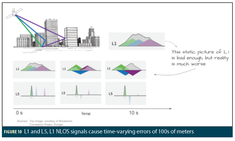
When you have one reflection you almost always have several, and with L1, these reflections cause overlapping correlation peaks. This is bad enough if you think of the static image you may be used to seeing.

But reality is much worse, different rays have slightly different Dopplers, and different phases, and they constructively and destructively interfere with each other, as shown in the snapshots over ten seconds. The peak of the correlator response varies over more than the width of the overlapping correlation triangles, that is: hundreds of meters. Because the satellite is moving, this happens even for a stationary receiver.

Thus, even with the 3D models, it is not possible to predict the received pseudorange at a specific time for overlapping NLOS signals. It is only possible to model it in a statistical sense. However, with L5 the situation is clearly different. We generally get separable correlation peaks, and so we can accurately model the NLOS pseudorange.

In summary: L5 will not solve the NLOS problem by itself. It simply makes the NLOS bias measurements more precise. while the biases are still present. But with 3DMA, this property becomes magic: we can correctly model the L5 channel, even with multiple reflections. and so 3DMA + L5 provides the solution we want for NLOS signals.

Deployment and Results

3DMA has been launched to 3 different clients and benefits many millions of users around the world.

The first client is GoogleMaps LiveView, which was launched in May 2020. Here, a server-side approach is used where an ML model processes building models and GNSS measurements at the backend, and sends results to the phone. This implementation provides the best urban performance due to larger processing power at the backend. In LiveView, Bluesky reduced GNSS WSS events by 90%.

The other 2 clients of 3DMA are the Android Fused Location Provider (FLP) and GNSS chipsets. Both use 3DMA corrections to improve their location accuracy.

The V1 GMS–Core implementations of 3DMA were launched in March 2020. In the FLP client, this implementation serves all phones with Android version 8 and higher, that is: 1.5 Billion phones. The GNSS chipset client serves all phones with Android version 10 and higher.

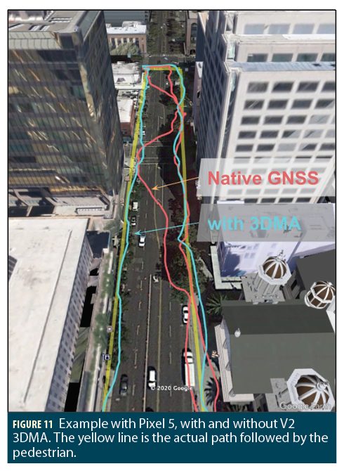
For battery and memory considerations, several optimizations are made to ensure 3DMA only runs when needed. E.g. Pedestrian mode, screen-on, and only in 3DMA Urban Geofences. For these clients, Bluesky reduces WSS by 50%, based on large scale validations, using Google-conducted tests, in 20 cities, on 4 continents, with ~1M data points. See Figure 11 for a working example

V2 of 3DMA was launched first to Pixel in December 2020 to Pixel 4a(5G) and Pixel5.

See Android developers blog [A 20]. V2 reduces WSS error by 75%. 3DMA V2 launched to the rest of the ecosystem (Samsung, Xiaomi, etc) in Q1 2021.

3DMA V3, launching in Q4 2021, will exploit the magic of L5. We consider this the endgame of 3DMA and urban GNSS wrong-side-of-street problems.

Acknowledgment

This article is derived from the Keynote Presentation at the ION ITM Meeting, Jan 2021. Video extracts of this talk can be found here: https://sites.google.com/corp/view/frankvandiggelen/videos.

References

(1) [MZ 78] “Accuracy on the order of 10m may be anticipated”

Source: PRINCIPLE OF OPERATION OF NAVSTAR AND SYSTEM CHARACTERISTICS (GPS SYSTEM DESCRIPTION) R. J. Milliken and C. J. Zoller, 1978. NAVIGATION, Journal of the Institute of Navigation, Volume 25, Number 2.

(2) [FCC] https://www.fcc.gov/general/enhanced-9-1-1-wireless-services

“Under Phase II, the FCC requires wireless carriers, within six months of a valid request by a PSAP, to begin providing information that is more precise to PSAPs, specifically, the latitude and longitude of the caller. “

(3) [G 16] “Simultaneous Localization and Mapping in Multipath Environments: Mapping and Reusing of Virtual Transmitters” C. Gentner et al. (DLR), ION GNSS 2016.

2D reflections of WiFi transmitters.

(4) [NG 16] “Direct Position Estimation Utilizing Non-Line-of-Sight (NLOS) GPS Signals” Y. Ng, G. Gao, ION GNSS 2016.

3D reflections of some NLOS GPS.

(5) [A 20] https://android-developers.googleblog.com/2020/12/improving-urban-gps-accuracy-for-your.html

Authors

Dr. Frank van Diggelen is a Principal Engineer at Google, where he leads the Android Core-Location Team. He also teaches GPS: he and Prof. Per Enge created an on-line GPS course, offered through Stanford University and Coursera and available on YouTube. He holds a Ph.D. in electrical engineering from Cambridge University, England.

Van Diggelen is a pioneer in Assisted GNSS, the technique that allows GPS to work in cell phones. He is the inventor of coarse-time GNSS navigation, co-inventor of Long Term Orbits for A-GNSS, and holds over 90 issued US patents on A-GNSS. He is the author of “A-GPS” and co-editor of “PNT in the 21st Century” (Morton, van Diggelen, Spilker, and Parkinson). He is President of the Institute of Navigation, a Fellow of the ION and the Royal Institute of Navigation (UK), and a member of NASA’s PNT Advisory Board.