
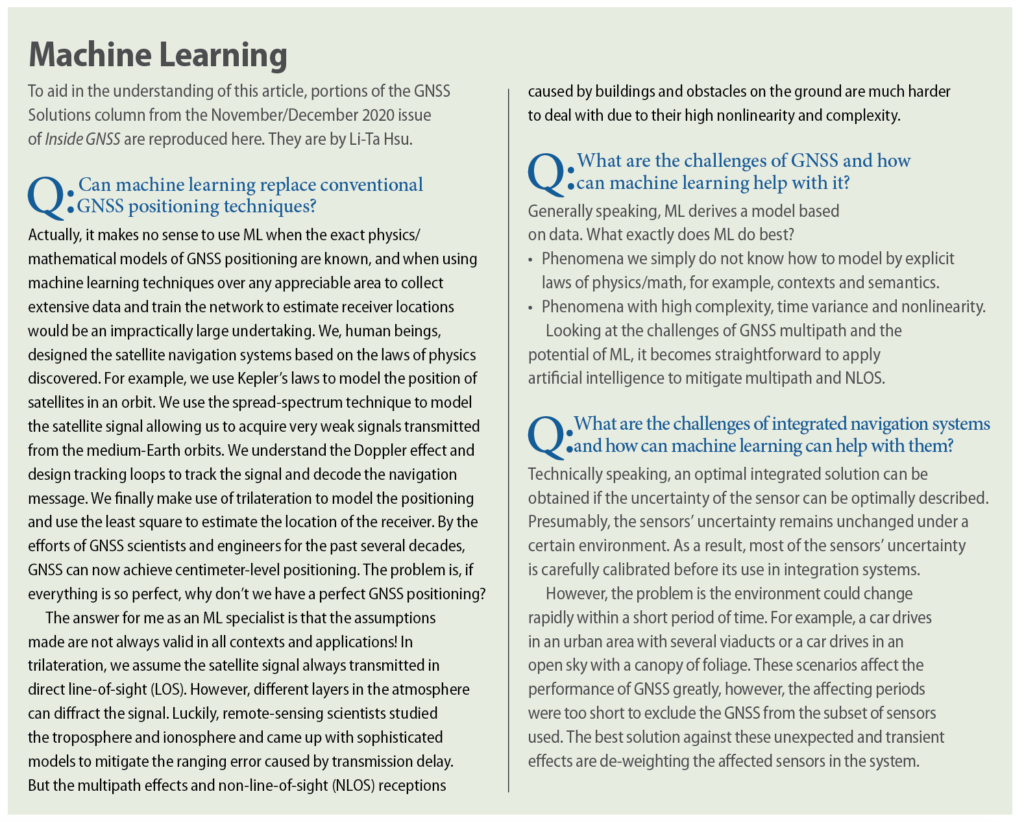
A novel method for improving the positioning accuracy of GNSS receivers exploits a machine learning (ML) algorithm. The ML model uses the post-fit residuals, which are readily available after the position computation from the position, velocity and timing (PVT) engine, adoptable by existing receivers without requiring any modification. The performance of this method, demonstrated using data collected with mass-market receivers as well as a Google public dataset collected with Android smartphones, shows the practicality of the concept.
GIANLUCA CAPARRA, PAOLO ZOCCARATO, FLOOR MELMAN
EUROPEAN SPACE AGENCY
GNSS receivers are prone to multipath errors. Increased receiver complexity, cost and power consumption constitute the main drawbacks of mitigation approaches relying upon designs of transmitted signals that allow a better multipath rejection and dedicated signal-processing techniques at baseband level. A mass-market receiver generally includes limited multipath rejection at antenna and baseband processing and applies some sort of filtering in the positioning engine. For instance, it is rather common to adopt a Kalman filter or pseudorange smoothing with phase measurements, as they produce a smoother and more accurate trajectory.
The errors related to atmospheric effects are instead usually compensated using atmospheric models or differencing with measurements from close-by reference receivers.
Recently, the use of machine learning with 3D mapping has been proposed to increase the accuracy of GNSS receivers. The performances achieved by this method are promising. The main disadvantage lies in the fact that it requires high-quality 3D maps to work. Moreover, these maps must be updated continuously to avoid introducing undesired biases.
Here, an approach that only needs information directly available in the GNSS receivers, and hence requires no information about the surroundings, attacks the multipath problem. The approach aims to create a ML model to be used after the positioning engine. This model estimates the positioning error exploiting the post-fit residuals and applies a correction to the PVT to compensate this error. The receiver still needs to receive the corrections from the trained model, but this model can be built based on GNSS results only. The ML regression acts as a sort of “adaptive filter,” able to cope with different environmental conditions automatically, properly adjusting the estimated position with a 3D error compensation. The ML feedback aims to map the directional pseudorange residuals to a 3D correction of the computed PVT.
The advantage of this approach is that it can be integrated in the current generation of receivers at software level, without requiring any hardware revision. It can even be deployed as a third-party service for the receivers that provide some basic additional information on top of the PVT.
Method Description
The GNSS receiver estimates its position by deriving the distance from at least four satellites with known ephemerides. The signals contain information on the satellite positions and the transmission time, which is referenced to the system time. The receiver records the reception time, according to its local reference clock, and then estimates the distance by computing the propagation time. This distance estimation is usually referred to as pseudorange, as it includes the geometric range plus several errors sources, e.g. synchronization error between the local reference clock and the system time, atmospheric effects and multipath. The pseudorange is the most used measurement adopted in the position estimation process.
The receiver position can be estimated by solving the navigation equations either using a weighted least square (WLS) solution or a Kalman filter. Due to the noise embedded in the input measurements, the best-fit of the state vector, which includes the position parameters, will have some differences with regard to the measured pseudoranges. The differences between the observed and modeled (from the estimated solution) measurements are usually referred to as residuals. These can be either the innovation residuals, if Kalman filter is used, or the pseudorange residuals, if LS/WLS is used.
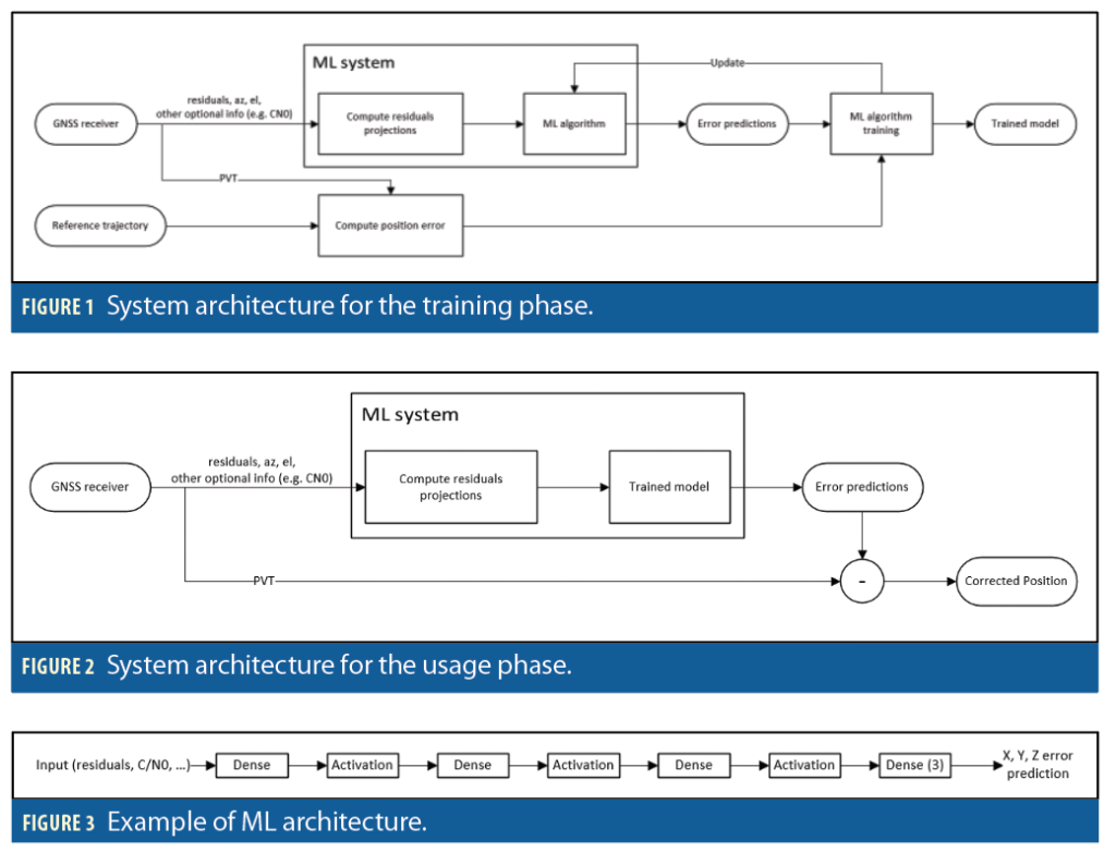
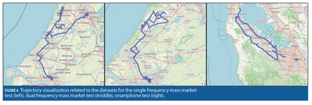
Our concept uses the residuals to train an ML model capable of predicting the 3D positioning errors, i.e. the differences between the estimated positions and the reference trajectory. The residuals are already present in the GNSS receivers: therefore, it does not require additional sensors for gathering external information. Figure 1 and Figure 2 present the detailed system architecture for the training phase and the usage phase.
The residuals, together with azimuth and elevation, can be projected into the navigation reference frame. The residuals are projected for all the signals used in the PVT computation.
These projected pseudorange residuals are the main input to the ML algorithm, which can be complemented by additional information, such as the carrier to noise ratio (C/N0) or other quality/reliability indicators. The ML model uses this information to estimate a positioning error. Depending on the application, the positioning error can be 3D or limited to the horizontal plane. It is possible to use any convenient reference frame. The approach described here is for a 3D positioning error, for instance in an East North Up (ENU) reference frame.
The training phase consists of finding a model that relates the residuals with the difference of estimated positions with respect to the reference trajectory, i.e. the position errors. The positioning error estimated by the ML model can then be subtracted from the position provided by the GNSS receiver, increasing the positioning accuracy.
When available, additional information can be included in the machine-learning model. This is left to future works. For instance, adding a label derived from the position indicating if the current area is rural or urban might help the ML algorithm to achieve better performances. Eventually, if the position itself (or a quantized version) is used in the ML model, the model can act as a sort of raytracing, because the model will learn how statistically the rays reflect in a certain environment, as a function of the azimuth and elevation. However, this would require an enormous amount of data. For this reason, this aspect was not taken into account for the time being. In this scenario, the algorithm would not be independent anymore from external information about the environment in which the receiver operates.
Proof of Concept
The concept has been tested with data collected from mass-market receivers. Three data analyses were performed:
• Single-frequency (SF) multi-constellation PVT solution from a mass-market receiver, used as a black box;
• Dual-frequency (DF) multi-constellation PVT solution from a mass-market receiver, used as a black box;
• Smartphone measurements (Google Smartphone Decimeter Challenge) using a single frequency PVT engine.
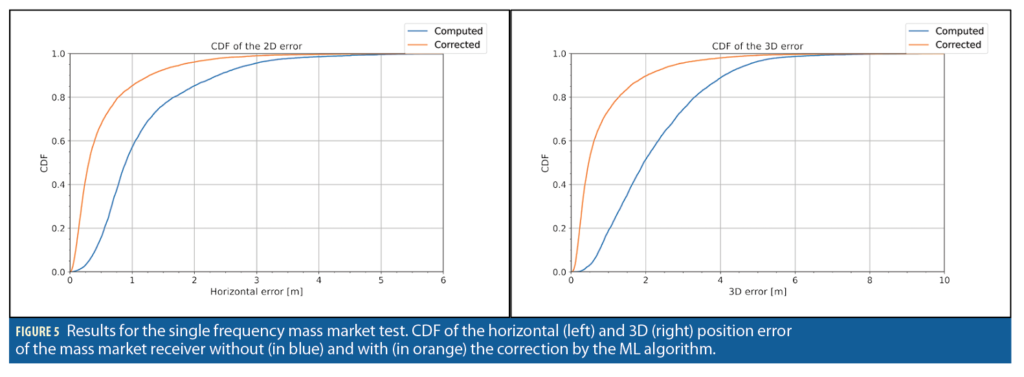
In the first two experiments, data was collected with mass-market receivers during test campaigns and field trials carried out in 2020-2021 in the Netherlands, targeting two main environments: a rural/open sky scenario and a deep-urban scenario in Rotterdam, (with parts of the data acquisition in highways). The datasets consist of several runs, for a total of about 117k, 175k and 95k epochs and are represented in Figure 4. A reference trajectory for ground-truth obtained with a high-end GNSS/IMU is also available for each trajectory.
In the experiments, each epoch was considered independently. Therefore, temporal correlation among epochs has not been exploited. The temporal correlation can be achieved by using a recurrent neural network (RNN), such as long short-term memory (LSTM), but this is left to future work.
The ML algorithm has been implemented as a neural network using Tensorflow. The neural network architecture is reported in Figure 3, showing an example with four layers, where the last one is fully connected, with three neurons (one for each direction of the coordinate system) and without activation, which provides the error estimation per component. Using a single ML model for all three components simultaneously (multi-target regression) allows capturing the correlations among the components. The algorithm can be tuned to work in different configurations. For instance, in the experiment with smartphone data, only the horizontal errors have been considered, leading to a final layer with only 2 neurons.
For the proof of concept, a neural network with six layers of respectively [2048, 2048, 512, 256, 32, 3] units was used. Each layer is followed by a rectified linear unit (ReLU) activation function. Limited optimizations of the neural network and of the training phase have been performed.
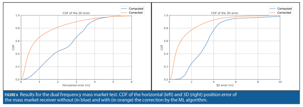
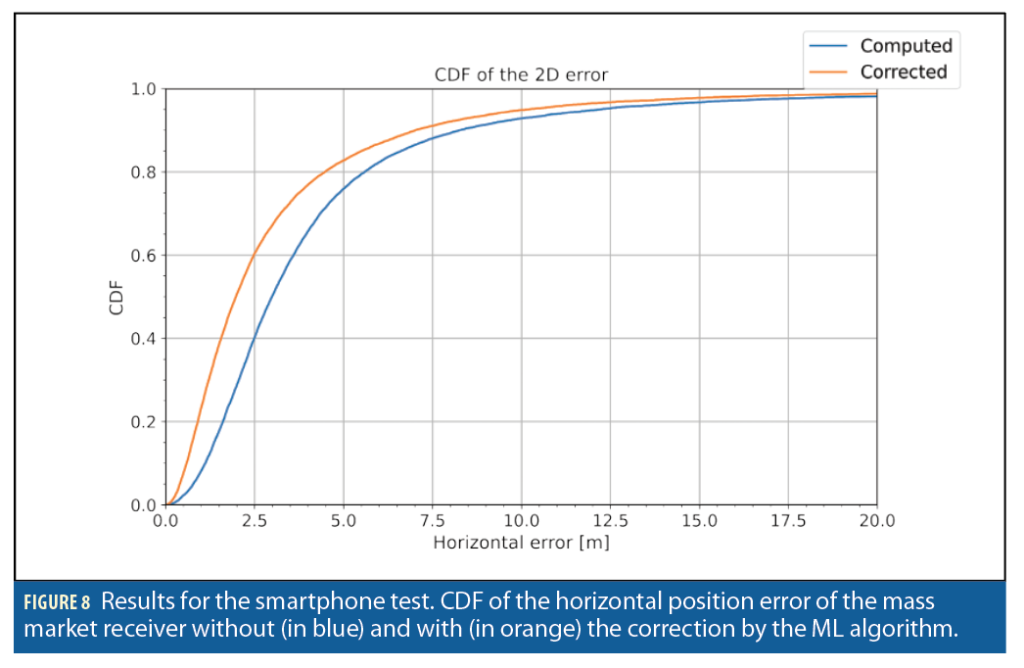
Within each dataset, 70% was used for training, 15% for validation, and 15% for testing. Figure 5, Figure 6 and Figure 8 show the results of the tests (taken from a random 15% of the dataset never presented to the ML model during training and validation), comparing the cumulative distribution function (CDF) of the positioning error with regard to the reference trajectory before and after the ML algorithm application on the PVT solution. Notably, the ML algorithm effectively improves the positioning accuracy.
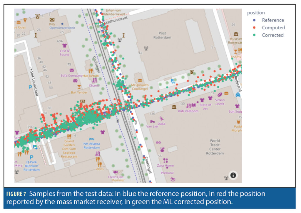
Figure 7 provides a visual representation of the results, taken from the Rotterdam city center area. The data are taken from the DF test. The positions from the reference trajectory are represented in blue, the positions computed by the mass-market receiver are depicted in red, and the one after the ML corrections in green. The corrected positions generally lie closer to the reference trajectory than the positions computed by the mass-market receiver.
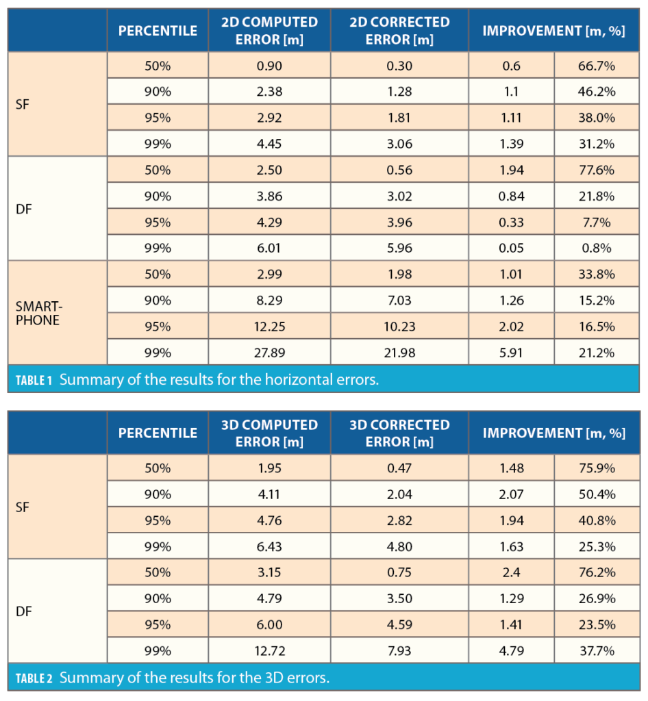
Table 1 and Table 2 report the summary of the results for horizontal and 3D errors respectively. The positioning errors are reported for different percentiles, together with the improvement in accuracy both in absolute and relative terms. It is interesting to note that at the 95th percentile, the improvement ranges between 7.7% and 38% for the horizontal errors, and between 23.5% and 40.8% for 3D errors.
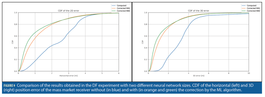
Network Complexity vs Performance
To assess the impact of the complexity of the neural network on the performances of the corrections, a smaller variant of the neural network composed by four layers of respectively [512, 256, 32, 3] units was tested. One iteration of the smaller model (NN1) requires around 50 µs on the laptop CPU (Intel i7-8650U) while the storage of the trained model parameters requires 2 MB. This allows it to be easily deployed to receivers. The bigger model (NN2) requires around 600 µs per iteration, and around 60 MB of storage. The results are reported in Figure 9. Note that NN2 achieves better results than NN1.
Conclusions
We have introduced the concept of machine learning corrections for improving the accuracy of the GNSS receiver’s positioning. The advantage of this method is that it does not require changes in the architecture of the GNSS receivers and can be deployed as a software service.
The concept has been demonstrated in three experiments using real-world data collected with mass-market receivers and smartphones, showing that it is possible to achieve a significant accuracy improvement, even with a neural network of modest size.
Future work will expand the dataset size, increasing also the variety of environments, to better assess the generalization of the ML model, and explore different ML architectures, e.g. investigating the benefit of LSTM for capturing temporal correlation among the epochs. Another interesting direction of research will be to explore the potential benefits for high accuracy positioning techniques, such as PPP (-AR) or RTK.
Acknowledgment
This article is based on material presented in a technical paper at ION GNSS+ 2021, available at ion.org/publications/order-publications.cfm.
References
(1) G. Fu, M. Khider, F. van Diggelen, “Android Raw GNSS Measurement Datasets for Precise Positioning,” Proceedings of ION GNSS+ 2020, September 2020, pp. 1925-1937.
(2) Martín Abadi, et al., “TensorFlow: Large-scale machine learning on heterogeneous systems”, 2015. Software available from tensorflow.org.
(3) F van Diggelen, “End Game for Urban GNSS: Google’s Use of 3D Building Models”, Inside GNSS, March 2021
(4) G. Caparra, “Correcting Output of Global Satellite Navigation Receiver”, PCT/EP2021/052383
Authors
Gianluca Caparra received a Ph.D. in information engineering from the Università Degli Studi di Padova, Italy. He is currently a radio-navigation engineer with the European Space Agency. His research interests include positioning, navigation, and timing assurance, cybersecurity, signal processing, and machine learning, mainly in the context of global navigation satellite systems.
Paolo Zoccarato holds a Ph.D. in science technology and measurements for space on precise orbit determination from the University of Padova, Italy. He worked at Curtin University as a PostDoc on PPP-RTK and in Trimble TerraSat GmbH on VRS and RTx. He is a radio-navigation engineer consultant at ESA/ESTEC, contributing mainly on real-time reliable high-accuracy positioning for different GNSS receiver types, sensors, environments and systems.
Floor Melman received a master’s degree in aerospace engineering from the Delft University of Technology (TU Delft), the Netherlands. He now works as a radio-navigation engineer at ESA/ESTEC. His main areas of work include PNT algorithms (in harsh environments) and GNSS signal processing.


