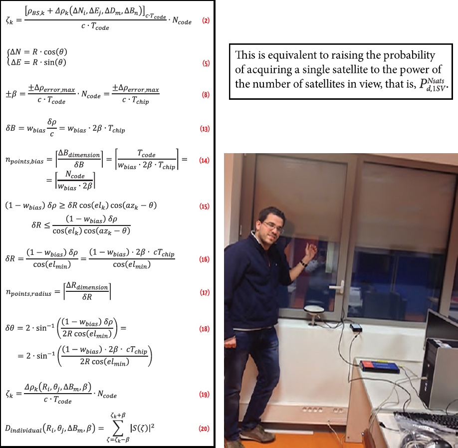
 Clockwise from left: (a) article equations, (b) the probablility of acquiring a single satellite to the power of the nyumber of satellites in view, (c) Indoor scenario of signal collection at ISAE navigation lab, Toulouse
Working Papers explore the technical and scientific themes that underpin GNSS programs and applications. This regular column is coordinated by Prof. Dr.-Ing. Günter Hein, head of Europe’s Galileo Operations and Evolution.
Working Papers explore the technical and scientific themes that underpin GNSS programs and applications. This regular column is coordinated by Prof. Dr.-Ing. Günter Hein, head of Europe’s Galileo Operations and Evolution.
The increased demand for geolocation services in dense urban environments poses a significant problem to satellite navigation systems (GNSS) due to the challenging task of receiving the extremely weak signals. Acquisition of GNSS signals in these harsh environments requires advanced signal processing techniques. Examples of such environments include forested areas found in many suburban neighborhoods, urban areas with tall buildings, and indoors.
In light of these limitations, recent efforts have pushed towards the use of high-sensitivity GNSS (HS-GNSS) receivers by using special signal processing techniques inside a receiver to extend the coherent and total signal integration time (See, for example, the articles by G. Lachapelle et alia and T. Pany et alia in the Additional Resources section near the end of this article. This desired accumulation of the signal can be performed over time intervals that far exceed the traditional 20 milliseconds, which allows for the detection of signals that are up to 100 times more attenuated than their nominal power.
To achieve such processing gains, two common approaches have emerged to improve the sensitivity of a GNSS receiver. The first approach is simply based on advanced algorithms of code delay, Doppler estimation, and data bit transition detection for a stand-alone receiver. Extended coherent integration can be accomplished also by using the pilot channels in the new GNSS signals. However, very difficult signal environments may make it impossible to decode the broadcast navigation data in the tracking mode and, therefore, no position fix will be computed.
The second approach involves the concept of assisted-GNSS (AGNSS), which receives assistance information from a server or a base station, to increase sensitivity by using the Doppler frequency of each satellite, reference time, initial position, ionospheric model, and ephemeris. (For further details on AGNSS techniques, the book by F. van Diggelen cited in additional resources provides a good introduction.) These two HS-GNSS technologies are now being used more commonly to improve availability of GNSS positioning in urban and indoor locations, but they are still not able to overcome the effect of severe degradations on accuracy and integrity of the navigation solution.
Another approach that is being extensively researched as a method to improve sensitivity in weak signal tracking involves processing all signals in view collectively, in what is known as vector tracking. This method combines the stage of signal tracking with the navigation module in a direct position estimation procedure.
Contrary to the conventional two-step position determination, the vectorized approach exploits the spatial correlation between signals from visible satellites, which are jointly processed to obtain the user’s position. The main rationale behind this approach is that the processing of weaker signals is facilitated by the presence of stronger ones. In most studies found in literature, nevertheless, each satellite signal is treated independently at the acquisition level. In this work, we focus on improving the application of the concept of collective processing at the acquisition stage (Figure 1).
R. DiEsposti introduced the application of the vectorial concept to acquisition in a 2007 paper (see Additional Resources), which proposed to coherently combine the detection metrics from all satellites in view. This concept relies heavily on assistance information, for the user to define a position and clock bias uncertainty range, and to receive the required data to carry out the methodology developed.
To cover the user 4D uncertainty space, this approach establishes a search grid in which each position and clock bias combination is mapped to the pseudorange and code phase for each satellite and a single detection metric is generated as a function of the expected user position and clock bias (Figure 2).
This approach was the subject of more recent studies that referred to it as collective detection. These studies refine the concept introduced by DiEsposti and improve upon it in several ways. In a 2011 article, P. Axelrad provides a thorough analysis of collective detection, demonstrating the performance improvement over traditional sequential acquisition techniques and using real signals.
These publications were also the first to propose a multi-iteration collective detection process, which begins with a rough search grid that covers the whole user position and timing uncertainty, and then is further refined in two more executions of the algorithm, successively reducing the uncertainty in both domains. This achieves a final search grid resolution that is quite fine, without needing to apply it to the whole uncertainty range.
More recent studies described in the thesis by J. Cheong addressed several different issues related to collective detection. These include different implementations of the algorithm, the effect of the search grid resolution on the computational cost of the collective detection methodology, and the effect on the positioning error of the timing accuracy supplied to the user.
Two significant advancements are also achieved in this thesis: the first one on the assessment of the performance of a combined GPS/Locata collective detection implementation, and the second one on the hybridization of collective detection with traditional sequential detection.
As shown in these publications, we can view collective detection simultaneously as a high-sensitivity (HS) acquisition method, by application of vector acquisition, and as a direct positioning (DP) method, providing a coarse position- clock bias solution directly from acquisition. As an HS acquisition method, collective detection is characterized by 1) sensitivity, and 2) complexity. As a DP method, it is characterized by 1) position error, and 2) time to first fix (TTFF).
All these metrics of performance can be linked to the position-clock search grid employed and, in this way, one of the biggest challenges in collective detection is the trade-off between resolution, which must be fine enough to allow good sensitivity and position error performance, and the number of points to be analyzed, which has direct repercussions on the algorithm’s complexity and TTFF.
In this article, we will address the optimization of the search grid to be employed in the collective detection search process. Our main goal here is to propose a methodology fulfilling two main requirements:
- systematic: the resolution to be employed in the clock bias-position searches is determined according to a set of input parameters; and,
- efficient: the search steps assure that the true signal code phase is not missed while avoiding excessively fine and computationally heavy search grids.
We name this new approach systematic and efficient collective acquisition (SECA). The advantage of the proposed method with respect to existing ones is precisely its systematic and efficient nature, given that previous proposals employ non-optimized, fixed-step search grids.
Our discussion here will also introduce the application of SECA, combining multi-constellation signals at the acquisition level. In this article, we use this approach for the case of a combined GPS/Galileo receiver. The integration of the collective and sequential signal detection approaches in a GNSS receiver can be achieved as proposed in Figure 3.
Collective Detection
In traditional acquisition architectures, the different signals are processed individually, which implies that the correct acquisition of each signal is dependent exclusively on its own signal strength and the receiver signal-processing techniques employed. Collective detection, on the contrary, follows a vectorial approach, in the sense that strong signals are acquired collaboratively to assist the detection of weaker ones.
Working Principle. The core concept behind collective detection is that the code phase search for all visible satellites is mapped into a receiver position-clock bias grid, implying that signals are not acquired individually, but rather all at once (collectively). The mapping of the signals’ code phase to the position-clock bias domain of a mobile station (MS), that is, a GNSS receiver in motion, is done differentially with respect to pseudorange measurements provided by a stationary base station (BS), as shown in Figure 4.
The difference in pseudorange from the MS with respect to the one measured by the BS for satellite k, Δρk, is given by:
Δρk = − cos(azk)cos(elk) ΔN – sin(azk)cos(elk) ΔE + sin(elk) ΔD + c ∙ ΔB (1)
where azk and elk are, respectively, the azimuth and elevation angles of satellite k as seen by the BS (considered to be the same as for the MS); ΔN, ΔE, and ΔD represent the 3D position displacement of the MS with respect to the BS in a North-East-Down (NED) local coordinate frame; and c ∙ ΔB is the pseudorange variation due to the clock bias of the MS, c being the speed of light.
For a hypothetical location ΔNi, ΔEj, ΔDm and clock bias ΔBn, the estimated code phase for satellite k, ζk, as would be seen by the MS at these coordinates is given by:
Equation (2) (see inset photo (a), above right, for all equations).
where Tcode stands for the signal spreading code period, Ncode is the number of code chips per period, and [∙]c∙Tcode represents the modulo c∙Tcode operation such that ζk [0, Ncode −1].
The individual detection metric for this satellite for these 4D coordinates is then calculated, for example, as:
Dindividual(ζk) = |S(ζk)|2 (3)
where S(ζk) corresponds to the correlation output of this satellite at the code phase ζk. Note that this detection metric is simply used as an example, as no impediment arises to employing other high-sensitivity detection metrics, such as the ones obtained through differential integration of the consecutive coherent outputs.
The individual detection metrics for all satellites obtained for this 4D point are then summed in order to obtain a single collective-detection metric for these hypothetical coordinates:
Dcollective(ΔNi, ΔEj, ΔDm, ΔBn) = ∑Dindividual(ζk) (4)
Once all possible combinations of the unknown parameters within their search space have been tested according to the collective detection principle, we can determine the set of values corresponding to the best estimation of the true MS position coordinates and clock bias.
Assistance Requirements for Collective Detection
In order to put the collective detection approach into practice, the MS requires that the following set of data be provided from the BS:
- coarse time and ephemeris — for computation of the expected satellite azimuth and elevation angles, as well as their velocity for compensation of the Doppler offset component due to satellite motion. Time synchronization within a few milliseconds (± 0.5 milliseconds to ± 2 milliseconds) should also permit direct despreading on secondary code sequences.
- reference frequency — for calibration of the MS oscillator, enables compensation of most of the oscillator Doppler offset component;
- BS position — for setting the initial MS spatial uncertainty; and,
- pseudorange measurements for all satellites in view as seen from the BS.
By compensating both for the oscillator and satellite-motion Doppler offset components, the factor that most affects the residual satellite Doppler is the user motion. This way, depending on the expected incoming signal powers and user dynamics, an exhaustive Doppler search may not be necessary.
Apart from the items listed here, the receiver may also be supplied with fine timing information (less than one millisecond accuracy), which may allow for a considerable reduction in its clock bias uncertainty.
Methodology of Implementation
The implementation of the collective detection principle typically involves four steps:
1. establish a spatial and timing uncertainty range for the MS with respect to the BS and define a grid to cover this uncertainty;
2. for each of the 4D points in the position-time search grid, employ the Collective Detection principle described previously;
3. perform an iterative refinement of the search grid’s resolution as the uncertainty in both domains is also successively reduced with each execution of the algorithm;
4. determine the position-clock estimates based on the results obtained.
We can accomplish the final step, which consists of the estimation of the MS coordinates, in several ways. The most obvious and straightforward is simply to establish that the 4D point that maximizes the collective detection metric is the most likely location-clock bias.
This, however, is not necessarily the most appropriate method, as the final search grid resolution may imply a very small step in code phase search from one point to the other, and a large area can be seen that is sure to contain the most likely coordinates, as in Figure 5.
Collective Detection as a Direct Positioning Method
Collective detection is capable of providing the user with a first coarse estimate of position and clock bias in situations where individual signals are too weak to be acquired/tracked or when the snap-shot signal is too short to be processed by standard methods. The accuracy of these estimates, however, is highly dependent on the visible satellite geometry, as in any other GNSS positioning algorithm, and available a priori information.
In the example shown in Figure 5, the signal strength is uneven; so, the collective detection metric is driven by the stronger signals. (This is reflected well in the nearly “diagonal” line visible in this plot.) If one of these stronger signals is from a satellite at a very high elevation, its code phase variation across the horizontal plane will be low, and a high ambiguity in the positioning may result if this signal is much stronger than the others.
The analysis of real scenarios shows that the positioning error of the collective detection approach depends, naturally, on the number of satellites visible, their geometry, and signal power. From previous publications it seems clear that, at best, the mean horizontal positioning error expected will be within a few tens of meters.
We should note, however, that this magnitude of positioning errors does not mean that the individual signals’ code phase is not being accurately estimated (within ±0.5 chips of the correct code phase), given that an error of 0.5 chips in the code phase estimation is equivalent to 150 meters in pseudorange for L1 C/A signals (and down to 15 meters for signals at higher chip rates, such as Galileo E5a and GPS L5). Therefore, a position error of 30 meters, for example, may still be within the correct code phase estimation region.
Collective Detection as a High-Sensitivity Acquisition Method
The objective of Collective Detection as a vector acquisition approach is to make use of the stronger signals to facilitate the acquisition of the weaker ones. The quantification of the performance of collective detection as an HS acquisition method, however, is not easy, as it is dependent on several factors, including the number of signals present and the relation between their powers.
As an example of its effectiveness, though, let us consider the hypothetical case that several signals are present at the same carrier-to-noise ratio, C/N0 (P. Axelrad). The probability of detection of a signal within Collective Detection in this case is roughly the same as the probability of acquiring a single signal by doing a number of non-coherent integrations equal to the number of signals present.
On the contrary, the probability of detection of the sequential approach is equal to the probability of correct acquisition of all signals simultaneously. This is equivalent to raising the probability of acquiring a single satellite to the power of the number of satellites in view, that is, (see inset photo (b), above right). The comparison results for 1 millisecond and 100 milliseconds coherent integration of a GPS L1 C/A signal are shown in Figure 6, where the full colored lines refer to the collective detection approach, the dotted colored lines respect the sequential one, and the full black line is the reference for one satellite signal.
As seen in this figure, the vectorial acquisition can be quite beneficial in the case where the signal strengths are very close to each other. In Figure 7, an example of application of the two acquisition techniques for signals at 35 dB-Hz is also shown for one millisecond coherent integration. In the plot for the Collective Detection approach, a clear peak around the user true location, (ΔN, ΔE) = (0,0), can be clearly seen, while naturally the individual signals are undetected on their own.
Collective Detection Search Grid Influence
The biggest drawback of collective detection highlighted in the technical literature is the potentially high number of points that need to be evaluated in order to have an acceptable resolution in the code search.
The clock bias dimension, in particular, can become very burdensome to search, given its large uncertainty and its direct one-to-one effect on the pseudorange and code phase. If a very fine resolution is directly employed in the search over the whole uncertainty range, the number of points to be analyzed becomes massive and this approach, impractical. Therefore, a compromise between sensitivity and complexity must also be made in collective detection.
The approach typically followed is to define an initial “rough” grid that covers the whole 4D uncertainty search space with a coarse resolution, and iteratively refine it until the desired resolution is achieved, while the uncertainty in all dimensions is continually reduced. The initial coarse grid resolution, however, needs to be carefully chosen, in order not to incur the risk of incorrectly estimating the uncertainty region to be analyzed in the following iteration.
To avoid this risk, two options can be employed: either the search resolution is fine enough to assure that the maximum estimation error in the code phase is under a half chip for every satellite or, alternately, use an averaging approach in which the grid allows an estimation error higher than half chip and the individual detection metric for each satellite is chosen as the average of the detection metrics within a certain range.
Both approaches have pros and cons, particularly in the trade-off between complexity and sensitivity. Clearly, the first approach involving a finer grid offers enhanced robustness in signal detection with respect to the second one, but it may also be much more computationally demanding.
The Proposed Method: SECA
The goal of the proposed SECA algorithm is to optimize the search grid employed in the 4D collective detection search process. The first step in the proposed algorithm is the redefinition of the local horizontal search from a North-East referential to a polar Rho-Theta. This way, we can write
Equation (5)
and (1) becomes
ρk(R, θ, ΔD, ΔB) = −R cos(elk) [cos(azk)cos(θ) + sin(azk)sin(θ)] + sin(elk) ΔD + c ∙ ΔB
= −R cos(elk)cos(azk − θ) + sin(elk) ΔD + c ∙ ΔB (6)
Furthermore, we neglect the vertical component for the time being, in order to obtain
Δρk = −R cos(elk)cos(azk − θ) + ΔB
= Δρposition + Δρbias (7)
Figure 8 summarizes the objective of the search grid definition described next for the horizontal position search. As shown in this figure, the resolutions to be employed in the search process are defined by a set of parameters that is also defined next. This applies to the clock bias resolution as well.
Search Grid Definition
In order to optimize the search grid, we start by defining the maximum code phase error in chips, β, that can be considered acceptable within the collective detection search process. Recalling the relation between the code phase and the differential pseudorange, this requirement is then translated to
Equation (8)
from which we obtain
Δρerror, max = β ⋅ c ⋅ Tchip = δρ/2 (9)
where δρ represents the resolution in the pseudorange to which corresponds the maximum code phase error of β chips. This resolution is then translated into the position-clock search step as
δρ ≥ δρposition + δρbias (10)
meaning that the sum of the steps in both dimensions cannot exceed the pseudorange resolution. In fact, none of the steps in position or clock bias should exceed the pseudorange resolution, but this is also implied by the above condition.
The partitioning of δρ can be divided between the two according to their effect on the positioning error, thus:
δρ = δρposition + δρbias = (1 − wbias) δρ + wbiasδρ (11)
where wbias ∈]0; 1[ is the weight of the clock bias step. Thus, δρposition and δρbias can now be expressed as functions of δρ and wbias. Starting with the bias component, defining δB as the resolution in the bias step, we obtain
δρbias = c ⋅ δB = wbiasδρ (12)
from which proceeds
Equation (13)
This resolution is then translated into a number of points to be searched by considering the total bias uncertainty. Assuming that no fine assistance information is available, the clock bias uncertainty is within a full code period of the incoming signal. Further assuming for the moment a GPS-only collective detection implementation, the clock bias uncertainty range, ΔBdimension, will then be one millisecond for the GPS L1 C/A signal. The number of points in the clock bias dimension, npoints,bias, is finally
Equation (14)
where stands for the nearest integer rounded towards +∞.
For the position uncertainty, starting with the radial Dimension
Equation (15)
The minimum values for the ratio on the right side of the above inequality are obtained when θ = azk, and the lowest satellite elevation from the set of satellites in view is considered this way:
Equation (16)
According to (16), the constellation geometry rises as a factor to take into account in the definition of the search grid resolution. The number of points to be searched for the radial dimension, npoints, radius, is then
Equation (17)
where ΔRdimension corresponds to the maximum horizontal search range.
This definition of the position uncertainty range also comes as more intuitive than the squared search range, as it is defined as a circle with the BS position as center and radius ΔRdimension. For the angular resolution, a similar reasoning can be employed to come up with
Equation (18)
According to this expression, the angular resolution is equally a function of β and of the lowest satellite elevation from the set of satellites in view. Furthermore, it is also a function of the search radius, being finest at the maximum radius. For the case R = 0 (the center of the grid), the resolution results as infinite, meaning that only one point (the center itself) is used for this uncertainty area.
From (14), (17), and (18), the influence of the value of β in the total number of points to be searched is well remarked. Given the difficulty of analyzing the total number of points for the angular search, the assessment of the relation between β and the total number of points has been verified in simulations to be on the order of 1/β3.
To summarize, the set of parameters that defines the search grid for the proposed SECA method (Θ) in Figure 8 is:
1. the code phase uncertainty to be considered for each candidate grid point, β. If this term is set too low, an excessive number of points may be obtained in the search grid.
2. the weight of the bias error component in the error allocation, wbias. If this is set too high, the error due to the clock bias becomes very significant due to the one to one impact on the pseudorange.
3. the maximum range uncertainty around the BS, ΔRdimension
4. the lowest elevation angle from the set of satellites in view, elmin.
The first two parameters can be freely set, the third one depends on the assistance, and the fourth, on the visible constellation and the mask angle.
Generation of Individual Detection Metrics
The value of β has a very important effect on the number of points to be searched. We previously mentioned that one way to handle a high code phase uncertainty in the collective detection search grid is to associate a range of code phases to each search point in an averaging process. This approach is followed, in order to be able to freely adjust the value of β.
*For each point in the search grid, the candidate code phase for each satellite is calculated as
Equation (19)
However, knowing that this code phase can be within ±β chips of the true code phase, the individual detection metric for each satellite is obtained as the sum of the detection metrics for range around the central code phase
Equation (20)
Search Grid Iterative Update
Again, if the value of β is set too low, we obtain a very high code phase resolution, but the number of points that will need to be considered grows considerably. This way, a more conservative value for β can be set at first, and then refined, as the position and clock bias uncertainties are also reduced.
Figure 9 provides an example of the application of the new algorithm through simulation. The true MS position is set to (ΔN, ΔE)= (−4000, 7000) and the clock bias to one kilometer. The chosen bias weight was 0.15, the minimum elevation angle considered was 30 degrees, and the radial uncertainty around the BS is set to 10 kilometers.
In this example, we chose an initial value of β = 5, which at each iteration is divided by 10. Three iterations are run so that β goes from 5 to 0.5 to 0.05. At each new iteration, the uncertainty in the clock bias and radial dimensions is made equal to the resolution of the previous iteration, and the resolutions of the new iteration are calculated using the new value of β and the new uncertainties. Table 1 shows details of the execution of the new algorithm.
A total of six strong signals are used for this simple illustration. The plots in Figure 9 show the collective detection metrics for each iteration at the most likely clock bias. The total number of points scanned is 52,030, considerably lower than the values found in literature, even not taking into account the vertical dimension in these methods.
Combined GPS/Galileo Collective Detection
With the advent of multi-constellation GNSS receivers, it is natural to foresee the application of collective detection in such context. In the experimental work described next we focus on the case of a combined GPS/Galileo receiver.
Considerations for Multi-Constellation Collective Detection.
One factor that must usually be taken into account when handling more than one constellation is the time offset between both constellations, in this case the GPS-Galileo time offset (GGTO). This time offset, however, is not an issue in the collective detection approach, given that its principle is to differentially compute the pseudoranges from the BS measurements. This way, all sources of error common to the BS and MS, including the clock offset of GPS satellites, do not need to be considered in (1).
Another factor to consider in a combined GPS and Galileo solution is that the Galileo E1 Open Signal (OS) spreading code period is four times longer than the GPS L1 C/A code. Depending on the input signal powers, this can produce disparities in the magnitude of the individual detection metrics between the two constellations.
The third factor to be considered in this context is that, given the longer Galileo E1 OS codes, the MS clock bias uncertainty is expanded by a factor of four with respect to the GPS-only case. This would, therefore, be directly translated to the number of points to be searched in this dimension as an increase by the same factor.
Finally, we must account for the presence of the secondary code sequence on the E1 pilot signal component either by limiting the coherent integration time to four milliseconds or by despreading the secondary code sequence. (We may assume that in most cases for HS acquisition, coarse time information should allow for directly despreading the secondary code chips.)
Handling Different PRN Code Durations in Collective Detection.
Given that the Galileo E1 OS spreading code is four times longer than the GPS L1 C/A signal, the MS clock bias uncertainty with respect to the BS must be extended to four milliseconds, instead of just one millisecond, as has been used so far in this article. Both signals have the same chip rate; so, one millisecond clock bias uncertainty only covers one quarter of the total Galileo code phases. On the other hand, by extending the clock bias uncertainty to four milliseconds, the GPS code phases will repeat themselves each millisecond.
This way, one practical solution is to “fold” the Galileo detection metrics twice, averaging the four points at “one millisecond distance” (1023 code phase) into just one. This will, once again, imply a reduction in sensitivity, but the computational savings are significant.
Real Data Results
To illustrate the combined GPS/Galileo collective detection process incorporating the SECA algorithm, we carried out an experiment at the Institut Supérieur de l’Aéronautique et de l’Espace (ISAE), in Toulouse, France. A receiver capable of receiving and handling both GPS and Galileo signals was setup as the BS, and a second receiver was used to collect raw data at a position close by the BS. The two sets of data were then post-processed to execute the collective detection approach.
Example 1: Open Sky Scenario. The radial uncertainty range around the BS was set to 10 kilometers. A total of 13 satellites were visible at the time of acquisition (9 GPS and 4 Galileo). For the acquisition of the Galileo signals, in this specific case, the two channels (E1B and E1C) are non-coherently summed after correlation.
Figure 10 shows the result of the application of the collective detection process with the all-in-view satellite set, considering a signal observation time of one code period for both GPS and Galileo. We applied a mask angle of 10 degrees, and the resulting geometric dilution of precision (GDOP) was around 1.8. Although the positioning error obtained was still on the order of tens of meters, the position uncertainty is greatly decreased, compared to the initial uncertainty of 10 kilometers radial.
In order to compare the performances of the sequential and vectorial approaches, weak signals are emulated by injecting noise into the correlation outputs of the MS receiver. This approach is validated by the Gaussian nature of the noise at the receiver input at the acquisition level. Figure 11 shows the results for the acquisition of all satellites in view for three different mask angle values.
Several conclusions can be drawn from these plots. The clearest and most expected one is that vectorial collective detection with SECA outperforms sequential detection in the detection of weaker signals. We also note that, for low injected noise powers, the performance of both approaches is close, even slightly worse for collective detection in some cases.
In terms of positioning error of the Collective Detection approach, the position errors obtained are always on the order of a few hundreds of meters. Comparing these errors with the ones reported in literature, we can conclude that this is the typical performance of collective detection. In any case, in the examples provided, the MS position uncertainty is decreased by one to two orders of magnitude with respect to the initial uncertainty (1E4 to 1E3 or 1E2) (Figure 12).
Example 1: Indoor Scenario. In this example, data was collected inside the building of the navigation lab at ISAE (see accompanying photo (c), above right) to illustrate the difficulty of acquiring the weak GNSS signals, even using the advanced processing approach of collective detection. In this experiment, the reference antenna was only a few meters away from the mobile user’s antenna. However, the collective acquisition was performed on a search space with a radius of 2.5 kilometers to reflect a realistic application scenario.
Both GPS and Galileo satellites were visible for the reference antenna, and all incoming signals were coherently integrated over four milliseconds to avoid dealing with data bit transition issues. The left plot of Figure 13 shows the number of detected satellites using a standard sequential acquisition algorithm for this data set and for a different number of noncoherent integrations.
The right plot shows the positioning error obtained with the proposed approach for the same data set and performing 10 noncoherent integrations. Accordingly, we observe that for the two cases of three satellites visible at Point 1 and Point 9 (i.e., successful sequential detection according to the left curve), the position error drops considerably.
We can see that, in most of the cases (i.e., eight out of ten), only two satellites were detected using sequential acquisition indoors; so, PVT could not be computed in these conditions. However, in the curve of the right-hand plot in Figure 13 we can see that SECA-aided collective acquisition enables computation of a rough position with only a few hundreds of meters of error, which is quite interesting and promising for achieving further improvement in future work.
As a result of this research, we believe that, for deep urban and indoor GNSS positioning, new concepts must be developed that depart from the classic two-step sequential processing.
Conclusions
Processing very weak GNSS signals in constrained environments is still a challenging task. The low received signal powers characteristic of these environments demand advanced signal processing techniques that take advantage of the maximum available GNSS information.
In this study, we analyzed the extension to signal acquisition using the vectorized signal processing approach known as collective detection. By processing all signals in view to the receiver simultaneously, detection of weak signals is facilitated given the spatial correlation between the different signals. Collective detection also provides the user with a coarse estimation of its position and clock bias with respect to a base station.
In this study we also introduced a new methodology for implementing collective detection, which we called “systematic and efficient collective acquisition” or SECA. We described the new SECA algorithm, highlighting both of its main characteristics. We also proposed an application of collective detection in a combined GPS/Galileo context.
The results demonstrate the feasibility of multi-constellation collective acquisition, profiting from the higher number of satellites that will be available in the future. Through the acquisition of real signals, both in open sky and indoor environments, it was shown that the new approach outperforms sequential detection in the acquisition of weak signals.
The proposed approach can be integrated into any existing receiver without the need to modify hardware but is naturally dependent on assistance data.
Navigation receivers will soon have more signals from more GNSS systems than anyone could have dreamed a few years ago. This new wealth of signal diversity and measurement redundancy could make collective detection a more robust means of increasing receivers’ sensitivity. In the theory of signal processing and estimation, the more measurements there are, the better the solution.
However, subtle considerations exist about how best to combine these measurements in the case of GNSS acquisition, including differences of code rate, data rate, Doppler shifts, structure and spectrum characteristics, and so forth. Thus, we need more research to address these questions related to the collaborative processing of multi-channels, multi-frequency and multi-constellation signals.
The results of the research presented here also show that the indoor case study needs different processing approaches. It requires advanced techniques and assistance data to perform long coherent integration by compensating for the signal carrier offset, which is not considered in this study.
Additional Resources
[1] Axelrad, P., and B. Bradley, J. Donna, M. Mitchell, and S. Mohiuddin, “Collective Detection and Direct Positioning using Multiple GNSS Satellites,” NAVIGATION, Journal of The Institute of Navigation, Vol. 58, No. 4, 2011
[2] Cheong, J., Signal Processing and Collective Detection for Locata Positioning System, PhD thesis, University of New South Wales, 2012
[3] DiEsposti, R., “GPS PRN Code Signal Processing and Receiver Design for Simultaneous All-in- View Coherent Signal Acquisition and Navigation Solution Determination,” Proceedings of the 2007 National Technical Meeting of The Institute of Navigation, San Diego, CA, 2007
[4] Esteves, P., and M. Sahmoudi, L. Ries, and M-L. Boucheret “An Efficient Implementation of Collective Detection Applied in a Combined GPSGalileo Receiver,” Proceedings of the 6th European Workshop on GNSS Signals and Signal Processing (SIGNALS 2013), Neubiberg, Munich, 2013
[5] Lachapelle, G., and H. Kuusniemi, D.T.H. Dao, G. MacGougan, and M.E. Cannon, “HSGPS Signal Analysis and Performance Under Various Indoor Conditions,” NAVIGATION, Journal of The Institute of Navigation, Vol. 51, No. 1, 2004
[6] Pany, T., and B. Riedl, J. Winkel, T. Wörz, R. Schweikert, H. Niedermeier, S. Lagrasta, G. López- Risueño, and D. Jiménez-Baños, “Coherent Integration Time: The Longer the Better,” Inside GNSS, November/December 2009
[7] van Diggelen, F., A-GPS: Assisted GPS, GNSS, and SBAS, Artech House, 2009


