What freeware or open-source software packages are available to support GNSS performance evaluations?

In the years since civil and commercial use of GPS and GNSS became common in the mid-1990s, a variety of software tools have been developed to perform offline analyses of GNSS performance and data collected from GNSS receivers. Some of these tools are part of commercial software packages such as Matlab [1] or STK [2]. This article focuses on tools that are freely available (as of early 2020) and are standalone or work with commercial software.

At least two different classes of GNSS analysis software exist, although some tools support multiple objectives. The first class includes tools that predict GNSS performance based on propagating GNSS satellite orbits and calculating GNSS performance factors at specific user locations and times based on the projected locations of GNSS satellites (“satellite geometries”). The second class focuses on analysis of previously-collected GNSS measurements converted into a standard data format. This article will focus on performance prediction, and a later article within this column will examine the processing of measurement data. Future articles in this column may also consider the use of software tools to emulate GNSS receiver functions in real-time and post-processing.

One of the original motivations for software to predict GNSS performance was simply to show the quality of future GNSS satellite geometry at specific places and times. In the early years of GPS, when the GPS constellation had fewer and shorter-lived satellites than it does now, periods of weak GPS geometries (either an insufficient number of visible and healthy satellites to compute a solution or a sufficient number but with poor Dilution of Precision, or DOP, which relates range measurement error to position and/or timing error) were not uncommon. However, absent a sudden change in the health of the GPS satellites, these periods could (and can) be predicted in advance.

Trimble Online GNSS Planning Tool

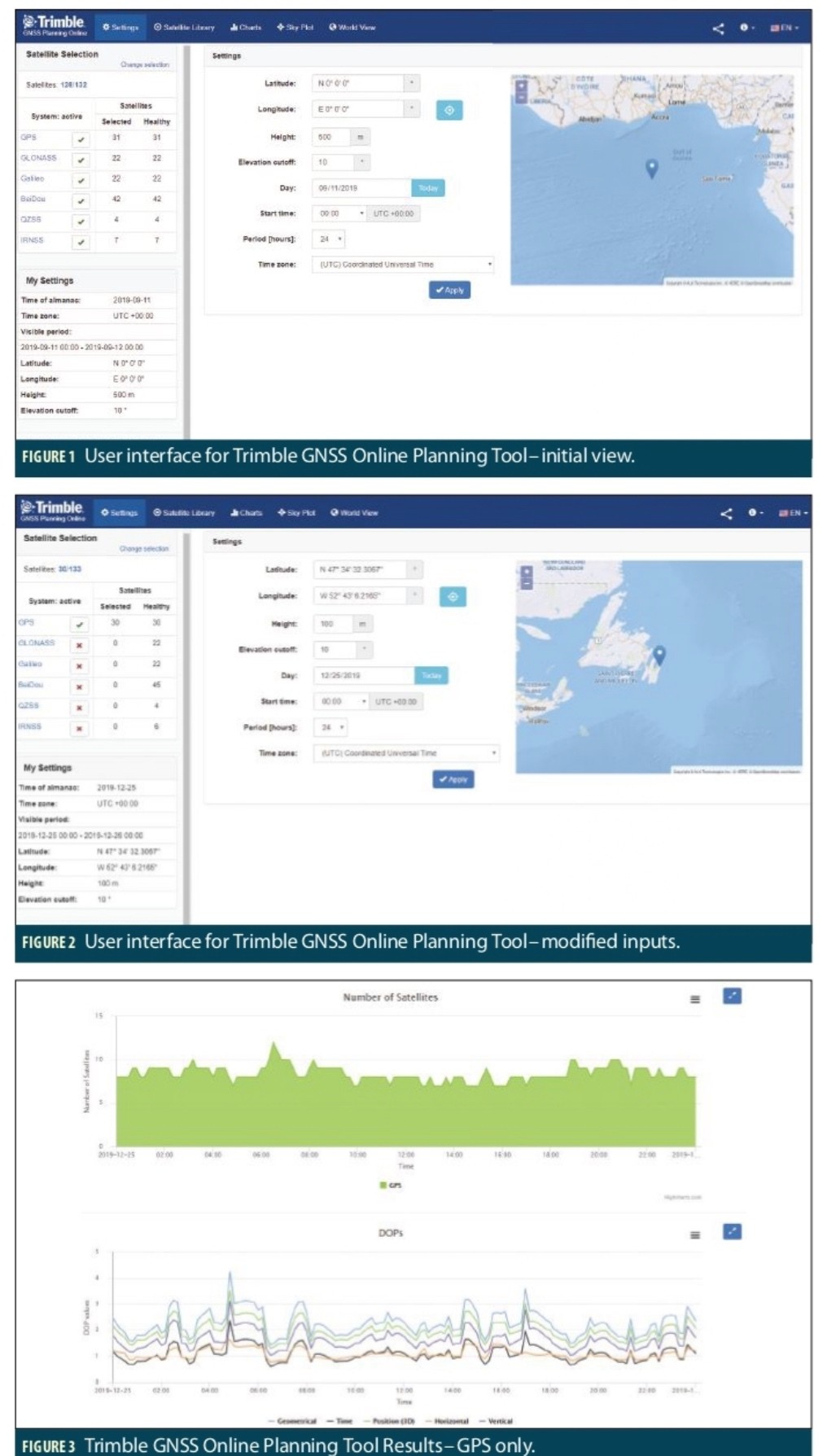
The Trimble Online GNSS Planning Tool available at [3] is useful because it is easy to access and run. It is an evolution of software previously provided by Trimble to help surveyors and other users of Trimble GNSS receivers identify the periods when GNSS satellite geometries would be good enough to support their applications. Figure 1 shows the screen presented to a user when first connecting to the website. The central window shows the default user location at the intersection of the equator and the prime meridian, the elevation angle cutoff (“mask angle”) for satellite visibility, and the time period to be simulated, while the left-hand screen shows the GNSS satellite constellations that can be used (or not used) as part of the performance prediction. All of these parameters are easy to change. The user location, for example, can be changed manually or by using the map in the right-hand window, while the usable satellites can be set by constellation or individually by satellite (using the “Satellite Library” menu tab). When constellations are selected to be used, all satellites marked as “healthy” by the latest almanac downloaded for that constellation are set to be used, while those marked as “unhealthy” are set as unused, but this can be changed on a satellite-by-satellite basis.

Figure 2 shows a scenario in which the user location has been changed to St. John’s, Newfoundland and Labrador, Canada, to investigate GNSS performance at higher latitudes. The left-hand window shows that only GPS satellites are used in this scenario and that 30 GPS satellites are healthy in the latest almanac. The time of interest is set to be the 24 hours following midnight Universal Time (UT) on Christmas Day, 25 December 2019 (note that local time in St John’s is 3 hours and 30 minutes behind UT in winter), and the elevation mask angle is left at the default value of 10 degrees.

Figure 3 shows two of the plots obtained by selecting the “Charts” menu item at the top of the screen. The upper plot shows the number of visible (and healthy) GPS satellites in view over the selected time period, and the lower plot shows five varieties of DOP values over this period, differentiated by different line colors. (The cursor can be placed at any point within the plot to read off exact numbers.) These plots show that between 7 and 12 healthy GPS satellites are visible over this period, and the PDOP (3D position DOP, not including time) varies between about 1.3 and 3.5, which is significant.

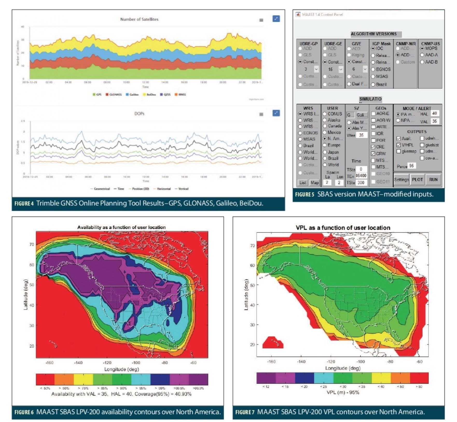
Figure 4 shows these same two plot results when the scenario is changed to use all satellite constellations. Now, as expected, the picture is very different, as GLONASS, Galileo, and BeiDou satellites also contribute significantly to positioning geometry (QZSS and IRNSS are used but are not visible at this location). The total number of visible and healthy satellites now ranges from 24 to 35, and PDOP varies between about 0.8 and 1.3. Not only are the DOPs much improved from before, but their variation with time decreases, making it much more unlikely that periods of unavailability will exist.

A key limitation of this tool is that all satellites are treated as having identical performance (both within and across constellations) except for being healthy or unhealthy, and key details such as satellite almanac parameters are fixed and cannot be changed. To perform more in-depth studies of GNSS performance, tools that allow access to these details and allow users to design their own performance metrics are needed.

Stanford MAAST

The Stanford Matlab Algorithm Availability Simulation Tool, or MAAST, is available at [4] and is a publicly-available set of source-code scripts that run within Matlab (and require a Matlab license to use). MAAST was originally developed about 20 years ago to predict Satellite-based Augmentation System (SBAS) performance (now “MAAST Version 1.4”) and has more recently been extended to support Advanced RAIM or ARAIM analysis (in “MAAST for ARAIM Version 0.4”). Dated but useful information on using and modifying MAAST software is contained in the “User’s Guide” and “Developer’s Guide” also available at [4]. Both versions of the MAAST source code can be modified and extended to support other GNSS applications.

The script “maast.m” within the SBAS version of MAAST currently runs a script called “maastgui.m,” which provides a graphical user interface (GUI) that allows users to change settings and execute performance simulations. This can be changed to instead run “maast_no_gui.m,” which allows these settings and parameters to be altered within the Matlab files. Figure 5 shows the control panel of the GUI after it has been altered to change certain parameters, including the values of UDRE (satellite clock/ephemeris error after SBAS corrections), GIVE (grid ionospheric vertical error after SBAS corrections), CNMP (receiver code noise and multipath error) models, user grid (covering all of North America in a grid of 2 × 2 degrees in latitude and longitude), GPS satellite almanac (the Yuma almanac for GPS Week 35 as of early December 2019, downloaded from the U.S. Coast Guard Navigation Center website at [5] and copied into the MAAST folder), the time update interval (one day at 300-second or 5-minute updates starting from the time of applicability of the almanac), the alert limits for SBAS-supported LPV approaches (HAL = 40 m, VAL = 35 m, corresponding to LPV-200, meaning LPV down to a 200-ft minimum decision height), and the output contour plots desired (vertical and horizontal protection levels, VPL and HPL, in addition to LPV-200 availability).

Pressing the “RUN” button at the lower right in the GUI starts a MAAST simulation with these parameters that generates the selected plots. Figure 6 shows the resulting contours of LPV-200 availability, which is defined as the probability at a given user grid location over the 288 simulated GPS geometries that VPL ≤ VAL and HPL ≤ HAL. The color scale at the bottom of the figure indicates the range of availability achieved within each contour, and these contours show how LPV-200 availability with these settings varies from above 99.9% (meaning in this case that all 288 geometries are available) near the center of the simulated reference station network to lower values farther away from the center of North America. The “Coverage(95%)” statistic at the bottom right indicates the percentage of user locations in the 2 x 2 user grid within the map that have availability of 95% or higher. It is less than 50% because the majority of the user grid is far away from the reference station network and does not expect to obtain high availability from SBAS.

Since vertical positioning is more challenging than horizontal positioning for GNSS, and because VAL is below HAL for LPV-200, the VPL ≤ VAL constraint on availability dominates the similar constraint on HPL. Figure 7 shows contours of 95th-percentile (95%) values of VPL from the same run that generated the availability results of Figure 6.These contours roughly (but not exactly) correspond to those of Figure 6, as the region in Figure 6 where availability exceeds 95% (light blue or darker) is similar to the region in Figure 7 where 95% VPL is below the VAL of 35 meters (light green or darker).

Note that, because the parameters shown in the GUI settings of Figure 5 (particularly the fixed values of UDRE and GIVE) are idealized and only roughly approximate actual SBAS values, these results do not mirror those achieved by today’s SBAS in North America (WAAS). Non-public versions of MAAST include the actual (proprietary) WAAS algorithms and give very accurate predictions for today’s WAAS as well as variations that are being considered for the future. The internal code of public version of MAAST described here can be modified to input WAAS UDRE or GIVE maps stored online, such as those provided in real time at the FAA NSTB website [6].

To show how to modify MAAST internal code scripts, it is easier to start with the ARAIM version mentioned above, which only runs in offline mode (starting with “main_maast_araim.m”). ARAIM is an evolution of traditional RAIM that uses multiple hypothesis solution separation to support real-time monitoring of multiple-satellite and constellation faults and is thus not limited to single-satellite faults, as is traditional RAIM. A detailed algorithmic description of ARAIM is at [7] (also see [Blanch, et al, 2015]).

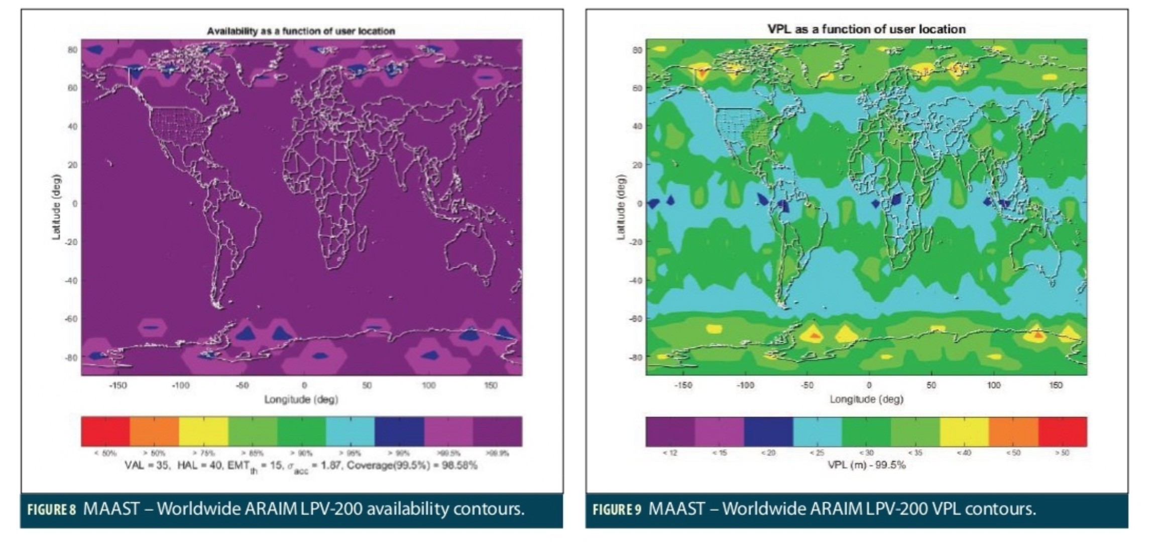
Figures 8 and 9 show the results of running the default ARAIM version of “main_maast_araim.m” except for two changes to reduce the granularity in the results. The first change (at lines 214-215) is to change the worldwide user grid to 5 × 5 instead of 10 × 10 degrees. The default ARAIM user grid covers almost the entire world because it is based on uncorrected (“standalone”) GNSS measurements and is not region-limited, as is SBAS. The second change (at line 225) reduces the interval between time epochs from 300 to 60 seconds, meaning that 1440 separate epochs are run to complete 1 day. Note that, unlike for SBAS, this ARAIM simulation uses a combination of 24 GPS satellites and 24 Galileo satellites to provide high availability of LPV-200 while also considering possible faults of all satellites in one constellation or the other.

The availability contours in Figure 8 show that the use of both GPS and Galileo (with the assumed default parameters) provides LPV-200 availability of 99.9% or better in most locations on Earth. Some high-latitude locations in both northern and southern hemispheres (at latitudes above the inclinations of GPS and Galileo satellite orbits) have availabilities as low as 99%. The contours of 99.5th-percentile VPL in Figure 9 show that it is these high latitudes that have the highest probability of VPL exceeding the 35-meter VAL for LPV-200. Within 60 degrees of the Equator, the 99.5th-percentile VPL appears to never exceed 35 meters.

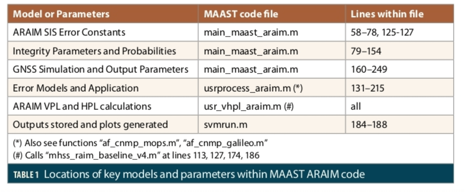
Again, the key advantage of the no-GUI version of MAAST is the ability to modify any of the parameters or algorithms that are described in the code. Table 1 summarizes where several key aspects of the ARAIM performance model are described in MAAST code files so that specific changes are easier to make.

Other Performance Analysis Tools

Several other GNSS analysis tools are freely available online, including the GPS Toolkit (GPSTk) [8] and RTKLIB [9]. Both of these are extensive and capable packages that support measurement analysis and position calculations based on data collected from GNSS receivers and stored in RINEX or other formats. A description of tools like these will appear in a subsequent article in this column.