Ionospheric delay is the largest source of range error for GPS Standard Positioning Service (SPS) users, at least during local daytime when solar emissions enhance these delays. However, ionospheric behavior in “mid-latitude” regions of the world is relatively benign, meaning that it very rarely has unusual variations. Delays as large as several tens of meters can be present in these regions, but they rarely change quickly over time and space. Correcting these delays using differential corrections from GNSS augmentation systems works very well as long as monitors are present to detect large spatial variations.<
However, in equatorial or low-latitude locations, unique physical characteristics of the ionosphere create both larger delays and much more unstable conditions on certain days and times of the year. As a result, even augmented GNSS struggles to obtain the same levels of performance that mid-latitude users are familiar with. These instabilities lead to both.
• scintillation of received GNSS signals, which degrades tracking performance and can cause loss of lock, and
• large spatial and temporal gradients in ionospheric delay that increase the residual errors after applying differential corrections.
Regions of the Ionosphere
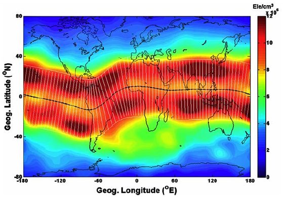
Figure 1 depicts the regions of the ionosphere on a global map (averaged data for 12:00-13:00 Local Time, or LT, over March and April 2007) and highlights their differences. The black line represents the magnetic equator, whose location with respect to the geographic Equator varies significantly with longitude. The equatorial region is typically defined to lie within ± 20 degrees of the magnetic equator. Within this region, ionospheric electron density is much higher than outside, as shown by the darkening red colors in Figure 1.
(This and other figures in this article are taken from papers that are fully cited in the captions and in the References section of the online version of this article, at insidegnss.com/equatorial.)
This region also has higher spatial variability in electron density levels. In contrast, the mid-latitude region between e 20 to 60 degrees north and south of the magnetic equator is much better behaved in terms of lower peak delays and lower variability. Beyond 60 degrees north and south of the magnetic equator lies the polar region, where delays are typically low, but ionospheric behavior is less stable and predictable than in mid-latitudes.
Note in Figure 1 that peak delay and variability within the equatorial region are not at the magnetic equator but are instead around 15 to 20 degrees north and south of it. This is important, as GNSS satellites whose ionospheric pierce points (IPPs—theoretical points in space where lines of sight from receiver to satellite intersect an assumed ionospheric altitude) lie within these latitude bands are those most likely to be impacted by the degradations described below.
Equatorial Plasma Bubbles
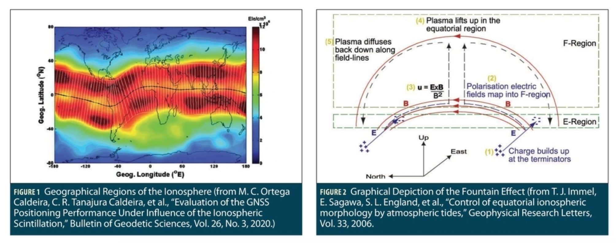
The atmospheric layers of charged particles making up the ionosphere result from the interaction of solar radiation with Earth’s magnetic field. Solar radiation both heats the upper atmosphere during local daytime and ionizes neutral particles. When these newly-charged particles are moved by upper atmospheric winds created by solar heating, they create electric currents and fields that interact with Earth’s magnetic field lines. The most important of these currents travels along the magnetic Equator and creates an eastward-directed electrical field. This combination of influences produces the Fountain Effect, in which charged particles are transported upward over the magnetic Equator, and as they reach higher altitudes, they move away from the magnetic Equator (following the electric field lines) while drifting downward due to gravity and pressure gradients. Recombination of these particles with free ions is more likely as they fall back toward Earth. A visualization of this process is shown in Figure 2. One result is the distribution of enhanced, irregular charged particle density shown in Figure 1, which is known as the Equatorial Ionization Anomaly (EIA).
Solar heating of the ionosphere changes over each day/night cycle, leading to a mostly eastward electric field with upward particle drift above the magnetic Equator during daytime and mostly westward electric field with downward drift during nighttime. However, around the day/night transition (roughly 1700 to 2000 LT in Brazil), “pre-reversal” of the equatorial electric field (and vertical drift) causes an abrupt peak of upward vertical drift to occur, and this can trigger unstable ionospheric dynamics in the early evening. In particular, irregularities known as Equatorial Plasma Bubbles (EPBs) can form at these times of day. When gravity waves from the troposphere reach the bottom side of the ionosphere and interact with eastward gravity-driven electric currents caused by pre-reversal, low-density plasma irregularities move upward due to the interaction of the electric and geomagnetic fields. The result is a bubble-like zone of depleted charged particles in the midst of larger regions of higher particle density that were previously enhanced by the Fountain Effect.
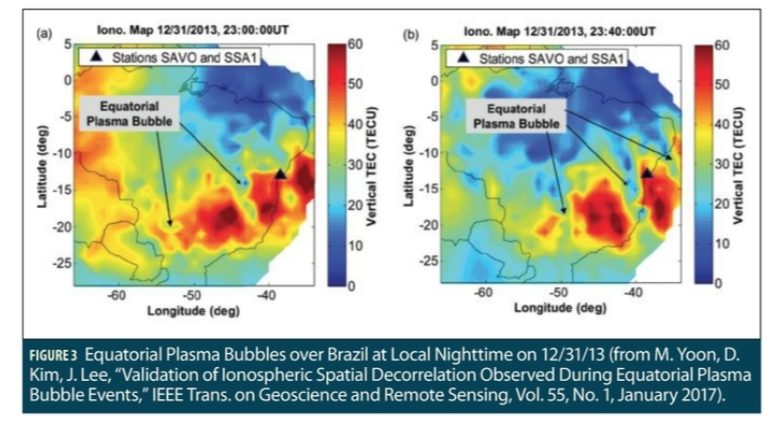
Figure 3 depicts EPBs over Brazil during local nighttime on December 31st, 2013 based on data collected by networks of GPS reference stations in South America. Eastern Brazil is 3 hours behind UT as given in the headers to both plots, so these plots show the period between 2000 and 20:40 LT. In the left-hand plot at 20:00 LT, at least two EPBs are visible as areas of blue shading (low vertical total electron content, or TEC) surrounded by regions of higher TEC in shades of yellow and red. In the right-hand plot at 20:40 LT, two of these bubbles are visible and are better defined. They have moved eastward along the direction parallel to the magnetic Equator, which is the typical direction of EPB propagation. The black triangle in both plots shows the locations of two nearby ground stations (SAVO and SSA1) in Salvador, Brazil, which were affected by these EPBs and spatial differences in slant (along the line of sight to the affected satellite) ionospheric delay as large as 31 TECU (about 5 meters at the GPS L1 frequency) over a separation distance of about 10 km.
EPBs are visible as small zones surrounded by the regions of high delay that occur at the peaks of the EIA about 15 to 20 degrees north and south of the magnetic equator, as suggested in Figure 1. Regions closer to the magnetic equator are not as disturbed
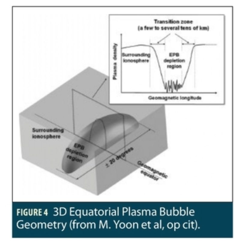
Figure 4 shows a 3D depiction of EPB geometry in a form that is useful for understanding EPB impacts on GNSS. The main graphic shows that EPBs typically span the entire equatorial region between ± 20 degrees of the magnetic Equator and usually move eastward along the direction of the magnetic Equator. The inset graphic at the upper right depicts the depletion of ionospheric delay inside an EPB (along with smaller irregularities in delay due to its unstable nature) surrounded by “transition zones” between outer regions of high delay. GNSS lines of sight that pass through these transition zones or the internal instabilities are likely to be affected by the effects discussed below.
User Impact: Scintillation
The regions of disturbed ionosphere shown in Figures 3 and 4 have plasma irregularities of various sizes. Irregularities of certain sizes (e.g., hundreds of meters across for GPS L1) will cause signals passing through them to fluctuate in amplitude and phase, leading to what is known as scintillation. Amplitude scintillation is typically measured by the S4 index, which is unitless and represents the normalized variance of received signal intensity over a short period (typically 60 seconds). Variations in phase measurements due to phase scintillation are measured by a similar (but not normalized) quantity σφ.
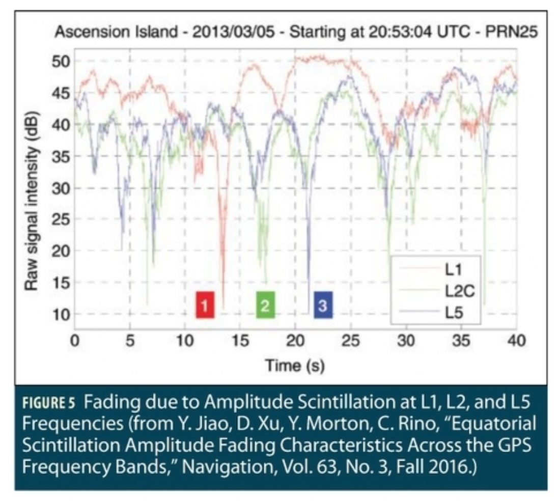
Amplitude scintillation in equatorial regions under disturbed conditions can cause signal fades of 15–20 dB or more and S4 values exceeding 1.0, which makes it difficult to continue to track the affected GNSS satellites. An example of strong fades is shown in Figure 5, which shows signal intensity from measurements of GPS satellite PRN 25 taken at Ascension Island (east of Brazil) on March 5, 2013. The 40 seconds of data shown include multiple sharp fades over 10 dB on all three transmitted frequencies (L1, L2, and L5) lasting from less than a second to several seconds. The strongest of these fades (beginning at 13 seconds) is on the order of 25 – 35 dB and occurs in quick succession on L1, L2, and L5, in that order of decreasing frequency. Scintillation is correlated with signal frequency, and longer fades sometimes overlap across frequencies, particularly on L2 and L5, which are not far apart. Despite this, using multiple frequencies for redundancy can help mitigate scintillation, especially when combining L1 with L2 or L5. Since these fades tend to be short, receivers that rapidly re-acquire after signal loss will be more robust.
While scintillation is possible throughout disturbed equatorial ionosphere, recent work shows the correlation between EPBs and strong amplitude scintillation. Looking at the multiple-EPB example in Figure 3, it is clear that several satellites might be affected by strong scintillation at the same time depending on the proximity of their lines of sight to the EPBs. Fortunately, even in the infrequent cases where this happens, the worst effect is loss of availability (unable to perform an operation) or continuity (having to abort an operation) as opposed to loss of integrity (unsafe or unbounded errors).
User Impact: Spatial Gradients
Even when GNSS signal tracking is retained, large differences in ionospheric delay over distances of 200 km or less is a major concern for GNSS augmentation systems. In the absence of indications not to use such measurements, this threatens user integrity. While both SBAS and GBAS have developed conservative threat models to bound these gradients in mid-latitudes it is more difficult to do this for equatorial regions without being very conservative and losing much of the value of providing augmentation.
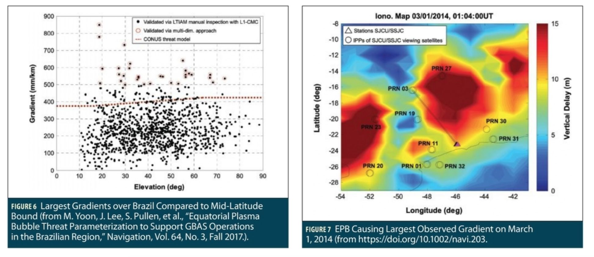
A preliminary threat model that attempts to bound worst-case spatial gradients in equatorial Brazil has been developed to support the GBAS facility at Galeão airport, Brazil. Figure 6 shows the results of the extensive collection of South American GPS ground receiver data between 2011 and 2015 that was used to generate the example in Figure 3. Each point within Figure 6 represents an observed and validated slant spatial gradient between two ground stations. The red dashed line shows the upper limit of the mid-latitude GBAS threat model, which has only been approached by the ionospheric storm of November 20th, 2003. The fact that many validated observations in Figure 6significantly exceed this line shows that much larger errors are possible in Brazil, and these errors make it difficult for the existing GBAS at Galeão to support Category I precision approach operations with high availability at local nighttime, when disturbed equatorial ionosphere may exist. The points shown with red circles in Figure 6 represent very large gradients that were subjected to additional validation tests because of their severe impact on GBAS.
Figure 7 depicts the EPB and ground to satellite visibility at the time of the largest observed and validated gradient of 850.7 mm/km at 01:04 UT on March 1, 2014. The two triangles toward the bottom show the locations of the two ground stations near São Jose dos Campos, Brazil (separated by about 10 km) that observed this gradient on GPS PRN 3. The two circles labeled “PRN 03” represent the approximate IPP locations for these two stations viewing this satellite. They appear to be at one of the transition zones of the EPB to the left of these circles, which is the cause of this very large gradient. The colors in this plot represent vertical delay as opposed to slant, and the difference between maximum and minimum delay is 15 meters at the L1 frequency, which represents an extremely strong depletion. Importantly, within one to three minutes of the time that the maximum gradient was observed on PRN 3, the same two stations also observed large gradients on PRN 19 (571.0 mm/km) and PRN 11 (465.0 mm/km), which also have IPPs in transition zones. Thus, very large range errors on multiple satellites are possible when the user-satellite-EPB geometry is particularly unfavorable.
Ionospheric Nowcasting and Mitigations
As explained above, single-frequency GPS and GNSS applications may be significantly degraded by ionospheric irregularities in equatorial regions on certain nights, particularly those near the peak of the 11-year solar cycle and near the spring and autumn equinoxes. A direct mitigation is to employ ground and user receivers that make use of L2 and/or L5 signals in addition to L1. When L2 or L5 measurements are available along with L1, “ionosphere-free” measurements can be computed that almost completely remove the influence of ionospheric delay (see [12] for an application of this to GBAS). However, as suggested by Figure 5, the scintillation that accompanies these disturbances may overlap and briefly knock out signal tracking on two frequencies. Even if only one frequency is affected, ionosphere-free dual-frequency processing would have to accommodate this temporary loss. In any case, full dual-frequency equipage among users and satellite providers is not expected before the latter part of the 2020s.
In the meantime, research on using GNSS station networks like those that generated the results in Figures 3, 6, and 7 to “nowcast” the presence and evolution of EPBs appears promising. In mid-latitudes, some GBAS installations use SBAS corrections to confirm that the ionosphere is not disturbed in the vicinity of the GBAS ground station IPPs. In one experiment (see References), a network of stations was used to estimate GBAS ionospheric threat model parameters. Nearby GBAS installations could use this information in real time to adjust the threat parameters that they must mitigate. In the case of EPBs, knowledge of their eastward propagation dynamics should allow stations to the west of GBAS installations to observe oncoming EPBs and alert the GBAS stations. When alerts are absent, protected GBAS installations would need to mitigate threat models much less severe than the worst case shown in Figures 6 and 7.
Summary
The space weather physics behind the ionospheric irregularities that appear in equatorial regions make the use of GNSS more challenging than it is in mid-latitudes. On some nights, the Fountain Effect creates irregularities that, when combined with updrafts of low-density plasma from the bottom to top-side of the ionosphere, leads to the formation of Equatorial Plasma Bubbles. These bubbles and the small-scale disturbances that accompany them produce both scintillation (leading to signal fades and potential loss of tracking) and large spatial gradients that can lead to large and unexpected errors in differential GNSS augmentation systems. In this environment, the use of multiple GNSS signal frequencies is recommended to provide signal redundancy and enable dual-frequency “ionosphere free” measurement processing. Development of techniques for using existing GNSS ground station networks to observe and alert augmentation systems of equatorial irregularities in near-real time is highly recommended.
References
[1] L. Sparks and E. Altshuler, “Ionospheric Storms of Solar Cycle 24 and their Impact on the WAAS Ionospheric Threat Model,” Proceedings of ION GNSS 2016. Portland, OR, September 2016. https://trs.jpl.nasa.gov/bitstream/handle/2014/46240/CL%2316-4420.pdf
[2] S. Datta-Barua, J. Lee, S. Pullen, et al., “Ionospheric Threat Parameterization for Local Area Global-Positioning-System-Based Aircraft Landing Systems,” AIAA Journal of Aircraft, Vol. 47, No. 4, July-August 2010. http://web.stanford.edu/group/scpnt/gpslab/pubs/papers/DattaBarua_AIAAJA_JulAug2010_Ionospheric_Threat_Parameterization_Local-Area_GPS.pdf
[3] M. C. Ortega Caldeira, C. R. Tanajura Caldeira, et al., “Evaluation of the GNSS Positioning Performance Under Influence of the Ionospheric Scintillation,” Bulletin of Geodetic Sciences, Vol. 26, No. 3, 2020. https://doi.org/10.1590/s1982-21702020000300014
[4] J. Sousassantos, L. Marini-Pereira, A. de Oliveira Moraes, S. Pullen, “GBAS Operation in Low Latitudes – Part 2: Space Weather, Ionospheric Behavior, and Challenges,” Journal of Aerospace Technology and Management, Vol. 13, 2021 (forthcoming). http://www.jatm.com.br/ojs/index.php/jatm/issue/archive
[5] Interface to Space: The Equatorial Fountain, NASA Scientific Visualization Studio, NASA/Goddard Space Flight Center, https://svs.gsfc.nasa.gov/4617. Accessed August 27, 2021.
[6] N. Balan, L. Liu, H. Le, “A brief review of equatorial ionization anomaly and
ionospheric irregularities,” Earth and Planetary Physics, Vol. 2, 2018. https://doi.org/ 2010.26464/epp2018025
[7] T. J. Immel, E. Sagawa, S. L. England, et al., “Control of equatorial ionospheric morphology by atmospheric tides,” Geophysical Research Letters, Vol. 33, 2006. https://doi.org/10.1029/2006GL026161
[8] M. Yoon, D. Kim, J. Lee, “Validation of Ionospheric Spatial Decorrelation
Observed During Equatorial Plasma Bubble Events,” IEEE Trans. on Geoscience and Remote Sensing, Vol. 55, No. 1, January 2017. https://doi.org/10.1109/TGRS.2016.2604861
[9] Y. Jiao, D. Xu, Y. Morton, C. Rino, “Equatorial Scintillation Amplitude Fading Characteristics Across the GPS Frequency Bands,” Navigation, Vol. 63, No. 3, Fall 2016. https://doi.org/10.1002/navi.146
[10] https://doi.org/10.1002/navi.203
[11] M. Yoon, D. Kim, S. Pullen, J. Lee, “Assessment and mitigation of equatorial plasma bubble impacts on category I GBAS operations in the Brazilian region,” Navigation, Vol. 66, No. 3, Fall 2019. https://doi.org/10.1002/navi.328
[12] M-S. Circiu, M. Meurer, M. Felux, et al., “Evaluation of GPS L5 and Galileo E1 and E5a performance for future multifrequency and multiconstellation GBAS,” Navigation, Vol. 64, No. 1, Spring 2017. https://doi.org/10.1002/navi.181
[13] S. Pullen, M. Luo, T. Walter, P. Enge, “Using SBAS Corrections to Enhance GBAS User Availability: Results and Extensions,” Proceedings of EIWAC 2010, Tokyo, Japan, November 2010. https://bit.ly/2UZUGTQ
[14] M. Caamano, J. M. Juan, M. Felux, et al., “Network-based ionospheric gradient monitoring to support GBAS,” Navigation, Vol. 68, No. 1, Spring 2021. https://doi.org/10.1002/navi.411


