A few studies (by universities and industry) have shown the feasibility of simulation of real-time digital intermediate frequency (IF) signals based on a graphics processor unit (GPU). And a couple of articles have also demonstrated use of a universal software radio peripheral (USRP)–based software-defined radio (SDR) as a simulator (in playback mode) in real test environments.
A few studies (by universities and industry) have shown the feasibility of simulation of real-time digital intermediate frequency (IF) signals based on a graphics processor unit (GPU). And a couple of articles have also demonstrated use of a universal software radio peripheral (USRP)–based software-defined radio (SDR) as a simulator (in playback mode) in real test environments.
However, to the best of our knowledge, all the most recent studies seem to share a lack of results in portraying the detailed performance of such simulators in presence of high-grade GNSS receivers. Moreover, opinions are divided as to the quality of USRP performance and their usability for high-grade GNSS receiver testing.
Nevertheless, this is an important aspect to consider for all potential users who consider the SDR approach as an alternative solution to conventional hardware-based simulation equipment.
The team of LASSENA (Laboratory of Space Technologies, Embedded System, Navigation and Avionic) of the École de technologie supérieure in collaboration with Skydel Solutions conducted a series of tests with a new SDR GNSS simulator. The purpose of the tests was to evaluate the real performances of the SDR simulation approach when used in conjunction with high-grade GNSS receivers.
This article presents the test methodology, results, and conclusions drawn from these tests. The first section will introduce the SDR GNSS simulator design. The methodology section describes the test setup and the approach employed for analyzing the test data. The results section presents the measurements that we obtained, along with their analysis.
SDR GNSS Simulator
The SDR approach has some advantages when compared with conventional simulators. Generally speaking, the conventional simulators use a dedicated hardware for high-rate signal modulation and a personal computer (PC) for low-rate computations.
Figure 1 schematically illustrates the most common architecture of conventional GNSS simulators. Low-rate processes usually deal with simulation of satellites orbit, receiver trajectory, atmospheric delays, antenna pattern, impairments, and so forth. The pseudorange, Doppler, and power per satellite are computed and serve as stimuli for processing in the hardware circuits.
The high-rate modulation is usually done in field-programmable gate array (FPGA) modules. Depending on the FPGA’s specific functionality, a number of dedicated channels per module cannot be changed for a given hardware design.
Conventional hardware simulators were used for GPS/GNSS receivers testing and validation from the beginning of GPS. The simulators brought repeatability and control to simulated satellite constellation and impairments. At that time, no other alternative but FPGA-based technology existed for high-rate digital signal processing to enable real-time simulation. For more than three decades, the conventional simulators evolved into a very precise and robust GNSS test equipment allowing for millimeter-level precision on simulated code- and carrier-based range measurements.
Dedicated hardware simulation approaches, however, have some disadvantages, perhaps the most important of which are a high cost per unit and reduced flexibility due to a slow product-development evolution as these types of simulators are typically deployed in low numbers. Adding new features or functionalities can be difficult and costly, as the programming of FPGAs requires special programming tools and skills. Also, in order to add additional signals or constellations, some or even all of the hardware has to be replaced, which may be very expensive and impractical.
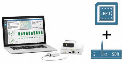
In contrast, a SDR GNSS simulator uses off-the-shelf products such as a PC equipped with GPU and USRPs. High-rate modulation is carried out on the GPU instead of the dedicated FPGA modules. GPUs are sold as mass-market products with relatively low prices. Meanwhile, as with integrated circuits, the processing power of GPUs follows Moore’s Law and doubles every 18 months. Moreover, the programming of such devices is based on general programming tools and does not require special skills, greatly facilitating the evolution and portability of the simulator.
As for USRPs, these universal SDR platforms are sold in large quantities and economies of scale keep the price low. Consequently, SDRs are constantly evolving, improving the RF signal quality and increasing the signal bandwidth.
Two modules comprise the SDR simulator under consideration (in turnkey configuration): 1) a PC or laptop and 2) a USRP. The two modules are connected via a high rate data link. To allow for different configurations and hardware connectivity, the data link can be either PCIe x4, PCIe x1, 10-gigabyte Ethernet, or 1-gigabyte Ethernet. The simulator is cross-platform and can run on Windows, Linux, or OS X operating systems.
The first module, the PC, simulates the selected GNSS constellations and executes all necessary computations to generate the high-rate zero IF GNSS baseband signal. The digital complex IQ data stream is then transmitted (via a high throughput link) to the USRP. This second module carries out signal pre-processing and filtering, and converts the zero IF baseband signal to RF.
The USRP is configured to have the signal’s power level per satellite at RF output as selected by the GNSS simulation scenario. The USRPs allow for single or multiple RF outputs. Figure 2 presents a generic block-diagram of the SDR simulator.
The PC does the low-rate computations on its CPU and the high-rate modulation on the GPU. Nowadays, off-the-shelf GPUs allow for hundreds of channels (satellites) to be simulated simultaneously with rates higher than 25MS/s per channel in complex (that is equivalent to more than 20 megahertz of bandwidth per channel) to support real-time simulation. The GPU by itself is a modular product and, if required, can be upgraded in the PC to increase the channel bandwidth or number of channels.
For SDR simulation, the USRP is basically used as a frequency up-converter to translate the zero IF baseband signal to RF. The main functional parts (in transmission) of the USRP are the digital-to-analog converter (DAC) and the frequency up-converter. Depending on the selected model, the USRP device may have one or several RF up-conversion channels.
The sample clock for all DACs is derived from the same reference clock, which can be internal or external. For multi-frequency simulation, multiple USRPs can be synchronised by an external 10-megahertz reference and triggered by the common one pulse per second (1PPS) signal.
The first versions of the SDR simulator employed in this study use a networked SDR that can transfer up to 50 MS/s of complex, baseband samples to and from the host computer for the single-frequency model and a high-performance, scalable USRP SDR platform for the dual-frequency model. With the former, the GPS L1 or GLONASS G1 signals are simulated with a signal bandwidth of 20 megahertz. With the latter model, the GPS L1 and GLONASS G1 signals for all visible satellites are simulated simultaneously with 20 megahertz (or more, if required) of bandwidth per constellation.
For the test purpose of this study, we selected the single-frequency SDR simulator with the GPS L1-only configuration. The simulator includes: 1) a MacBook Pro, circa mid-2012, with i7-quad core and an NVIDIA GeForce GT 650M GPU, 2) the networked USRP SDR with a WBS RF daughterboard and 3) an external 10-megahertz oven-controlled crystal oscillator (OCXO) reference clock. (Note that a lower performance PC model could also be used without any performance degradations.)
Methodologies and Test Setup
A straightforward approach for achieving a coarse estimate of the simulated signals’ precision is to observe the behavior of the high-grade GNSS receiver stressed with the simulator and then analyze the raw data.
The precision of the standalone position as well as the code and carrier phase measurements represent a combined contribution of the performances of the SDR simulator and the GNSS receiver itself. Nevertheless, this provides a good indicator as the performances of high-grade receivers nowadays allow for better than one-millimeter resolution on the carrier and a couple of centimeters on the code measurements.
The team selected two high-grade GNSS receivers for precise measurements and raw data logging. Two types of scenario were created: static and dynamic with slow motion on a circle (radius = 50 meters and speed = 3 meters/s).
Figure 3 shows the test setup. The simulated signal (via a passive three-decibel splitter) is evenly distributed between two identical high-grade GNSS receivers. The satellites are simulated with equal power (no power variations with elevation angle) and the carrier-to-noise density ratio (C/N0) at the receivers’ input is set to 46 dB-Hz (to minimize the noise contribution of the receiver). In order to avoid additional errors due to a mismatch of atmospheric models between the SDR simulator and the receiver, the ionospheric and tropospheric delays were turned off on both.
The methodology for signal analysis is inspired by that described in the article by P. F. de Bakker et alia, although adapted to the present case. Essentially, the analysis is based on the code and carrier phase measurements, sometimes called observations in single- and double-difference formations. We also measured the stand-alone position estimate and analyzed the accuracy in two and three dimensions against the simulated one.
In general form, the observations are defined as per Equation (1) and (2):
P = r + cΔtrec − cΔtsat + T + I + Mp + τp + εp (1)
Φ = r + cΔtrec − cΔtsat + T + I + Mφ + λN + τφ + εφ (2)
where P and Φ are pseudorange and carrier phase accumulation, r is the geometric range, c is the speed of light, Δtrec and Δtsat are receiver and satellite clock errors, T and I are tropospheric and ionospheric delays, Mp and Mφ are code and phase multipath, τp and τφ are instrumental code and phase delay, and εp and εφ are random code and phase error (Let’s call the last variable phase noise).
Code Phase Estimate
We selected two different approaches for the code estimate: 1) using a double-difference (DD) technique (based on measurements from two receivers) and 2) through code-minus-carrier observations (based on measurements from one receiver).
In the first approach, the code phase noise is estimated through single- and double-difference formation. Considering the measurements for two receivers (A and B), we obtain:
Pam = r + cΔta − cΔtm + T + I + Mmpa + τpa + εmpa (3)
Pbm = r + cΔtb − cΔtm + T + I + Mmpb + τpb + εmpb (4)
The subscript a and b indicates measurements for receiver A and B, respectively and the superscript m, the m-th satellites. Pma,b is code pseudorange, r is geometric range, cΔta,b represents receiver clock errors, cΔtm is satellite m clock error, T and I are tropospheric and ionospheric delays, Mmpa,b is phase multipath, τmpa,b are instrumental phase delay, and εmpa,b is code phase noise.
Assuming that no multipath M, exists in the measurement, the single-difference (SD) range calculation to the satellite m is obtained as:
SDmpab = Pam − Pbm = cΔtab + τpab + εmpab (5)
where cΔtab = cΔta − cΔtb, τpab = τpa − τpb, and εmpab = εmpa − εmpb
To form the double difference, a second satellite n is selected for the SD:
SDnpab = Pan − Pbn = cΔtab + τpab + εnpab (6)
DDmnpab = SDmpab − SDnpab = εmpab − εnpab = εmnpab (7)
To estimate the variance of the code phase noise for a single receiver, we have to consider that the variance of a DD computation is approximately four times that of a single receiver, thus:
VAR(εmnpab) ≈ 4(1 − [ρε]SD) ⋅ VAR(εa) (8)
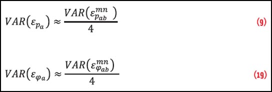
The [ρε]SD is the correlation coefficients for the SD formation. We assume that, for a single difference, no correlation exists between the phase noise of the two receivers, therefore, the correlation coefficient [ρε]SD ≈ 0. Based on this assumption and considering the same model of receivers and the same signal-to-noise ratio (SNR), the phase noise variance is given as
Equation (9) (see inset photo, above right)
In the second approach, the code phase noise can be easily estimated trough code-minus-carrier observations to the same satellite as follows:
P − Φ = ΔIρ−ϕ + ΔMρ−ϕ − λN + Δτρ−ϕ + Δερ−ϕ (10)
In this computation, the common code and carrier phase measurements parameters (r, cΔtrec, cΔtsat and T) are eliminated. Furthermore, for our particular case, we assume that ΔIρ−ϕ = 0 and ΔMρ−ϕ = 0 (that is, no ionospheric delay and multipath in the simulated scenario) and Δερ−ϕ ≈ ερ as the phase noise is about an order of magnitude lower than the code noise. Next, a low-order polynomial p(t) is fitted to the code-minus-phase computed data to remove slowly changing components.
With those considerations and without losing accuracy, code-minus-carrier becomes:
VAR((P − Φ) − p(t)) ≈ VAR(ερ) (11)
Carrier Phase Estimate
Traditionally, the carrier phase noise is estimated through SD and DD measurements. Considering those measurements for two similar receivers (A and B), we obtain:
Φam = r + cΔta − cΔtm + T − I + Mmϕa + λNam + τϕa + εmϕa (12)
Φbm = r + cΔtb − cΔtm + T − I + Mmϕb + λNbm + τϕb + εmϕb (13)
The subscript a and b indicates measurements for receiver A and B, respectively, and the superscript m, the m-th satellites.
The other terms in (12) and (13) are:
- Φma,b, carrier phase accumulation,
- r is geometric range,
- cΔta,b, receiver clock error,
- Δtm, satellite m clock error,
- T and I, tropospheric and ionospheric delays
- Mmϕa,b, phase multipath
- τϕa,b, instrumental phase delay
- εmϕa,b, carrier phase noise.
Considering that the ionospheric simulated delay is not applied (I = 0) and no multipath are simulated, the SD to the satellite m is obtained as
SDmϕab = Φam − Φbm = cΔtab + λNmab + τϕab + εmϕab (14)
To form the DD, a second satellite is selected for the SD:
SDnϕab = Φan − Φbn = cΔtab + λNnab + τϕab + εnϕab (15)
DDmnϕab = SDmϕab − SDnϕab = λNmab − λNnab + εmϕab + εnϕab (16)
We remove the cycle ambiguities λNmab and the cycle slips by inserting a fit polynomial p(t) into Equation (16), to obtain the following:
DDmnϕab − p(t) ≈ (εmϕab − εnϕab) = εmnϕab (17)
Again here, to estimate the variance of the carrier phase noise for single receiver, we have to consider that the variance of the DD formation is about four times the variance of a single receiver:
VAR(εmnϕab) ≈ 4(1 − [ρε]SD) ⋅ VAR(εϕa) (18)
where [ρε]SD is the correlation coefficients for the SD formation. Assuming that, for an SD, there is no correlation between thermal noise of two receivers, then the correlation coefficient [ρε]SD ≈ 0. Based on this assumption, and considering the same model of receivers and the same SNR, the variance of carrier phase noise becomes:
Equation (19) (see inset photo, above right)
Test Results and Analysis
The tests were repeated five times for each of the static and dynamics scenarios, and data was logged for 35 minutes. We processed the data based on the previously described methodology, which produced the results for code and carrier phase’s measurements presented in Table 1 and Table 2. Figure 4 and Figure 5 contain the results for the code and carrier phase noise (for static and dynamic tests) as a function of time. The results for the stand-alone receiver positioning error in static and dynamic tests are presented in Figure 6 and Table 3.
The measured code (using double-difference as well as in code-minus-carrier techniques) and carrier phase noise in the presence of the SDR simulator is in the range of the receivers’ precision (less than three centimeters for code and less than 0.4 millimeters for carrier). The results for stand-alone positioning are correlated with the code measurements. Based on these results, the SDR simulator allows for high-grade receivers’ testing at the limits of the precision defined by the receivers’ manufacturer.
The test results presented here were compiled based on GPS L1 C/A code only. We believe that the same approach can be applied to other type of signals and constellations. In fact, it is inspired from methodology used for Galileo signal analysis described in the de Bakker et alia article cited earlier.
Nevertheless, it can be concluded that the measurements will be somehow limited in precision by the receiver itself. For example, based on the specifications of the selected receiver, the code and carrier phase measurements for GLONASS G1, G2, and GPS L2 are expected to be almost twice the value for GPS L1 C/A. For the same reason, it is expected that the code and carrier phase measurements for GPS L5 will be close to values obtained for GPS L1 C/A.
Conclusion
In general, the SDR simulator is a very attractive solution due to its flexibility, the ease of integration with existing hardware (e.g. USRPs), and its affordability. On the other hand, people raise concerns about the performances of SDR simulators applied for real testing, especially for high-grade receivers.
This article has tried to answer those concerns, adopting a straightforward approach by jumping directly into the real use-case: simulation of precise GPS L1 signals. The raw measurements from two high-grade GNSS receiver were used as indicator of the simulated signal’s quality. The test results show that the phase measurements in the presence of the SDR simulator are better than 3 centimeters for the code and 0.4 millimeters for the carrier. The quality of simulated signals is also confirmed by the precision of the position estimates in stand-alone mode.
This study clearly confirmed that real-time SDR simulator, based on USRP, can achieve the level of precision suitable for high-grade receivers testing
Acknowledgment
The authors would like to thank Canal Geomatics and Philippe Doucet personally for their substantial support for the GNSS equipment. Also, the authors would like to thank the team of LASSENA for support in simulation and data collection.
Additional Resources
[1] Bartunkova, I., and B. Eissfeller, “Massive Parallel Algorithms for Software GNSS Signal Simulation using GPU,” in Proceedings of the 25th International Technical Meeting of The Satellite Division of the Institute of Navigation (ION GNSS 2012), Nashville, TN, pp. 118–126
[2] Brown, A., and J. Redd, and M. Dix, “Open Source Software Defined Radio Platform for GNSS Recording and Simulation.” Navsys Corporation, 2013
[3] Brown, A., and J. Redd, and M.-A. Hutton, “Simulating GPS Signals: It Doesn’t Have to Be Expensive,” GPS World, no. May, 2012, pp. 44–50
[4] de Bakker, P. F., and C. C. J. M. Tiberius, H. van der Marel, and R. J. P. van Bree, “Short and zero baseline analysis of GPS L1 C/A, L5Q, GIOVE E1B, and E5aQ signals,” GPS Solutions, vol. 16, no. 1, pp. 53–64, January 2012
[5] Li, Q., and Z. Yao, H. Li, and M. Lu, “A CUDA-Based Real-Time Software GNSS IF Signal Simulator,” in China Satellite Navigation Conference (CSNC) 2012 Proceedings, J. Sun, J. Liu, Y. Yang, and S. Fan, Eds. Springer Berlin Heidelberg, 2012, pp. 359–369
[6] Misra, P., and P. Enge, Global Positioning System: Signals, Measurements, and Performance. Lincoln, Mass.: Ganga-Jamuna Press, 2010
[7] Novatel, Inc., “Enclosures FlexPak6” specifications
[8] Zhang, B., and G. Liu, D. Liu, and Z. Fan, “Real-time software GNSS signal simulator accelerated by CUDA,” in 2010 2nd International Conference on Future Computer and Communication (ICFCC), 2010, vol. 1, pp. V1–100–V1–104


