
Accurate and reliable timing and synchronization can be an enabler of diverse new applications in datacenters. Accurate clocks across different nodes make possible key functions like consistency, event ordering, causality and the scheduling of tasks and resources with precise timing. In this article the authors take a close look at scalable and traceable time for datacenters using GNSS and White Rabbit.
In finance and e-commerce, clock synchronization is crucial for determining transaction order: a trading platform needs to match bids and offers in the order in which they were placed, even if they entered the trading platform from different gateways. In distributed databases, accurate clock synchronization allows a database to enforce external consistency and improves the throughput and latency of the database.
NTP, the popular clock synchronization protocol via internet, is cheap and easy to deploy, but its accuracy is typically in the millisecond range. The Precision Timing Protocol (PTP) provides an accuracy of around 100 ns in a local, fully “PTP-enabled” network. If the network hardware is not fully PTP-enabled, synchronization accuracy can degrade by a factor of 1,000. Both NTP and PTP perform poorly under high network load.
White Rabbit (WR) is a collaborative project for the development of a new Ethernet-based technology to ensure sub-nanosecond synchronization and deterministic data transfer. The project uses an open source paradigm for the development of its hardware, gateware and software components. Core hardware designs and source code are publicly available.
In this article we discuss the combined usage of GNSS and WR for timing and synchronization in datacenters. The topics of GNSS-to-WR phase alignment and GNSS calibration are addressed. An error budget is also developed to support traceability analysis from the timing solution at the user end node to a reference time scale such as UTC.
White Rabbit and its Integration with GNSS
The WR project was initiated at CERN in 2008 to synchronize different processes in its particle accelerator network. One of the main aims of the project is to deliver such functionality while using – or extending where needed – existing standards. To achieve sub-nanosecond synchronization WR utilizes Synchronous Ethernet (SyncE) for syntonization (frequency transfer), and IEEE 1588 Precision Time Protocol (PTP) to communicate time. A two-way exchange of the PTP synchronization messages allows precise adjustment of clock phase and offset. The link delay is known precisely via accurate hardware timestamps and the calculation of delay asymmetry. WR extends PTP in a backwards-compatible way to achieve sub-ns accuracy. WR was originally conceived for synchronization of more than 1,000 nodes via fiber or copper connections of up to 10 km, but coverage of longer distances has been already achieved.
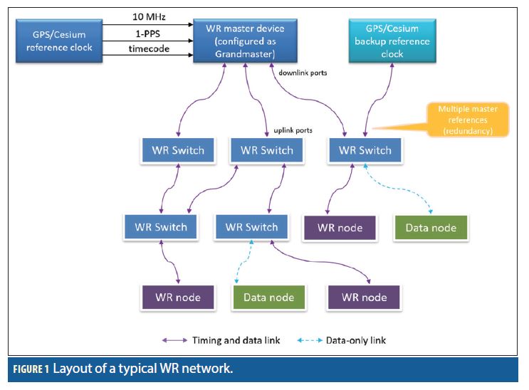
Figure 1 shows the layout of a typical WR network. Data-wise it is a standard Ethernet switched network, i.e., it follows a typical Ethernet tree or ring topology where any node can talk to any other node according to IP address and network protocol mechanisms. Regarding synchronization, there is a hierarchy established by the fact that switches have downlink and uplink ports and a master/slave relationship. A switch uses its downlink ports to connect to uplink ports of other switches and discipline their time. The uppermost WR switch in the hierarchy is usually called the “grandmaster”. The grandmaster receives its notion of time through external One Pulse Per Second (1PPS) and 10-MHz inputs. In this article we will assume that the top-level timing signals come from a GNSS receiver.
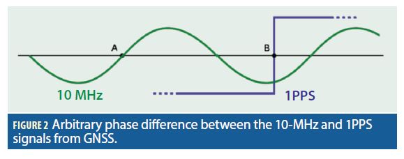
A correct phase alignment between GNSS and WR timing signals is essential for an unbiased and deterministic time distribution downstream. A typical GNSS receiver provides the time reference through its output 1PPS signal. The output 10-MHz frequency signal from GNSS “follows” the 1PPS coherently, i.e., the derivative of the 1PPS phase in time is consistent with the output frequency. However the phase relationship between the two signals is normally arbitrary. This is depicted in Figure 2, where B represents the rising edge of the 1PPS signal (which actually determines the time), and A represents the nearest zero-crossing of the 10-MHz frequency signal. The time difference A-B is not deterministic and can change after receiver power cycles and possibly also after GNSS signal interruptions.
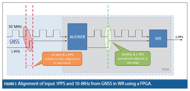
Furthermore, a typical WR grandmaster uses as main reference its input 10-MHz frequency and “locks” onto it continuously. The input 1PPS is only used at start-up to determine the nearest zero-crossing of the input frequency signal. Afterwards, the 1PPS is no longer used. Thus the time origin for WR is actually the initial zero-crossing of the input frequency signal, not the input 1PPS. This can result in a synchronization error between GNSS and WR of up to 50 ns (half the 10-MHz wavelength).
To overcome this problem, we have developed a new device (called “DOWR”) that integrates seamlessly a GNSS receiver and a WR grandmaster. The GNSS receiver is based on an industrial single-frequency GPS chip. The DOWR incorporates a novel method to continuously align the WR phase to the 1PPS from GNSS, using a dedicated FPGA module (shown in Figure 3). In this way the unknown phase relationship between the 1PPS and 10-MHz signals from GNSS becomes irrelevant. A small residual mis-alignment between the GNSS and WR 1PPS signals remains after applying this scheme. This offset is constant after start-up, and is strictly bounded within ± 1 ns.
GNSS Timing and its Calibration
GNSS timing receivers generate a precise 1PPS timing signal aligned to GNSS system time or to Coordinated Universal Time (UTC) as disseminated by GNSS. In the case of GPS, system time is called GPS Time (GPSt), and GPS’ dissemination of UTC is based on UTC(USNO), which is the UTC realization from the U.S. Naval Observatory. In a very simplified explanation, a GPS receiver estimates the instantaneous receiver clock bias (i.e., the clock offset versus GPSt or UTC) from its PVT solution using pseudoranges and navigation messages. The receiver then advances or delays electronically its internal clock signal accordingly in order to generate a 1PPS signal aligned to GPSt or UTC.
GNSS calibration is a well-established practice inside the metrological community. Indeed, the GNSS signal experiences a delay when traveling across the GNSS antenna, the antenna cable, and the receiver itself. The total delay of the chain, reflected in the output 1PPS, can reach a few hundred ns, with the major contributor being normally the delay of the antenna cable. When using GNSS for time transfer between national UTC laboratories, the calibration of the “receiver chain” (antenna + cable + receiver) is an essential task to properly compare atomic clocks and time scales in different countries at the ns level.
GMV has recently collaborated with the European Space Agency (ESA) and the Royal Observatory of Belgium (ROB) in a project called AKAL, to consolidate a procedure for absolute calibration of time-transfer GNSS receiver chains (see Garbin, et alia, Additional Resources). Absolute calibration consists in measuring the signal delays by means of simulated signals produced by signal generators: a GNSS simulator for the receiver, and a Vector Network Analyzer (VNA) for the antenna and the antenna cable. Absolute calibration of GNSS receivers has been gaining interest inside the timing community due to the low uncertainty level that can be achieved, and also due to the need of having a reference calibrated receiver, especially in a multi-GNSS context including the new Galileo and BeiDou signals. The uncertainty attainable from absolute calibration is in the order of 1 ns for the whole chain.
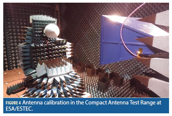
The absolute calibration of the antenna in AKAL is done in the Compact Antenna Test Range (CATR) at ESA/ESTEC, shown in Figure 4, thus benefiting from a large anechoic chamber. For the emitting antenna, a Standard Gain Horn (SGH) antenna is used. The calibration of the delay of the single SGH is done by means of using two identical SGHs and halving the resulting delay.
Regarding the GNSS receiver itself, absolute calibration is done by means of a GNSS signal simulator, where one can eliminate all atmospheric effects, as well as any multipath and environmental interference, and one can generate signals synchronized with the same clock being fed to the receiver. The output signal of the GNSS simulator needs first to be calibrated to estimate with low uncertainty the delay of the incoming signal in the receiver.
The calibration of antenna cables is usually not cumbersome. Their delay can be easily measured by means of a time interval counter, injecting a 1PPS signal at one cable end, and recording the difference with the output 1PPS from the other cable end. The attainable uncertainty is well below the ns, and is only slightly less accurate than using more sophisticated equipment such as a VNA.
Unlike metrological time transfer, in industrial GNSS timing applications the calibration of the receiver chain is often ignored. This can lead to timing biases of up to a few hundred ns. Unlike time-transfer receivers, industrial receivers do not normally have connectors for an external reference clock (frequency and 1PPS inputs), only the output 1PPS signal derived from GNSS is accessible (generated from an internal, inexpensive clock). A simplified way to calibrate an industrial receiver chain is by measuring the time difference between its output 1PPS and the 1PPS from the reference clock of a UTC timing laboratory. In 2017, two such receiver chains were sent by GMV for calibration using this method to PTB (Physikalisch-Technische Bundesanstalt), the German national metrology institute. Each chain is composed of an industrial single-frequency GPS receiver and an inexpensive patch antenna. The calibration was based on the measured differences between the 1PPS generated by the receivers (i.e., GPSt as determined by the receiver from pseudorange measurements) and the 1PPS of UTC(PTB), the German realization of UTC. The calibration uncertainty reported by PTB is 2.5 ns, which takes into account the uncertainty in the difference between UTC(PTB) and the GPSt generated by the receiver’s 1PPS, and also the errors in the GPS solution (mainly the residual ionospheric error).
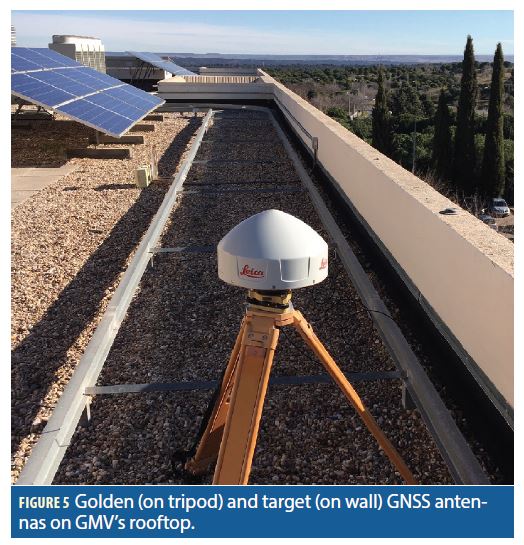
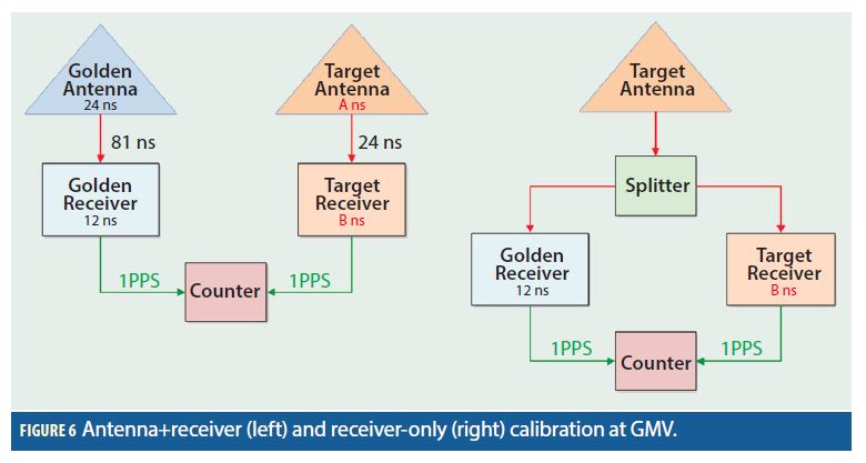
UTC laboratories do not always offer such calibration services to the general users. An alternative is to use an existing absolutely calibrated receiving chain as a reference for the industrial receiver, and measuring the time difference between their output 1PPS signals. The detailed procedure is explained in the following paragraphs. To define and test the procedure we have used as reference an absolutely calibrated receiving chain. We therefore first calibrated a “golden” time-transfer receiver chain, following the AKAL procedure at the ESTEC laboratory, and measuring the antenna, receiver, and antenna cable delays separately. The golden chain was then installed back at GMV. As a target receiver chain we have used one of the two chains calibrated at PTB in 2017. In this way we can compare the results of the two independent calibration methods. We installed the golden and target antennas on GMV’s rooftop, as shown in Figure 5. The detailed setup is sketched in Figure 6. The delays of the two antenna cables involved were measured beforehand using a time interval counter.
Precise coordinates were calculated for each antenna using real-time kinematic (RTK). We configured the two GPS receivers’ PVT in an identical way (as far as possible given that they are different models), i.e., fixed position, GPS-only using C1 code, 5-degree elevation mask, Klobuchar model, and the 1PPS aligned to GPSt. In this way the output 1PPS signals from the two receivers should match except for a bias due to the different chain delays, and fast variations due to the relative 1PPS generation uncertainty (“jitter”), which are assumed to be zero on average and thus not adding a calibration error as long as a data span of enough duration is used.
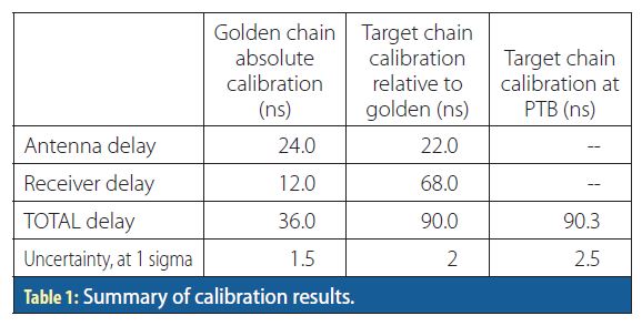
The combined delay of antenna plus receiver in the target chain is first measured (A+B in Figure 6, left). The time difference measured in the counter between the 1PPS of the golden chain and the 1PPS of the target chain over one hour is shown in Figure 7. Notice that, as expected, the 1PPS difference is fairly stable, with a standard deviation of 1.8 ns due mainly to the relative jitter of the 1PPS from the two receivers. When the delays of the two antenna cables are subtracted, the resulting combined delay of antenna and receiver in the target chain (A+B) is 90 ns. This matches very well with the value measured at PTB in 2017 (90.3 ns), considering that the two methods are totally independent.
Additionally, we can measure separately the receiver-only delay of the target chain (B in Figure 6, right). In order to do this we install the golden and target receivers on a common antenna (for example the target one) using a splitter. From the counter, a similar plot is obtained (shown on the right of Figure 7). The resulting delay for the target receiver (B) is 68 ns. Since the combined delay of antenna and receiver in the target chain (A+B) is 90 ns, we can conclude also that the delay of the target antenna (A) is 22 ns. A summary of the results is shown in Table 1.
The uncertainty of the proposed relative calibration method is tentatively estimated to be around 2.0 ns, derived from the nominal uncertainty in the absolute calibration of the golden chain (1.5 ns in GPS C1, from AKAL). It is important to notice that other than the absolutely calibrated golden chain, the calibration procedure of the target chain can be carried out by means of a counter (alternatively an oscilloscope), which is inexpensive equipment in comparison to absolute calibration equipment (VNA and GNSS simulator). Furthermore, once a target receiver chain has been calibrated in factory by the proposed method, it can be used as reference to calibrate additional chains using the same relative procedure.

Testing GPS in Combination with White Rabbit
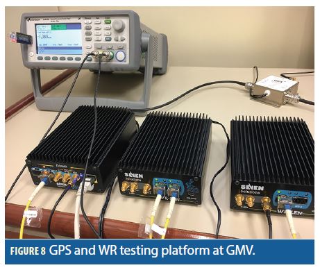
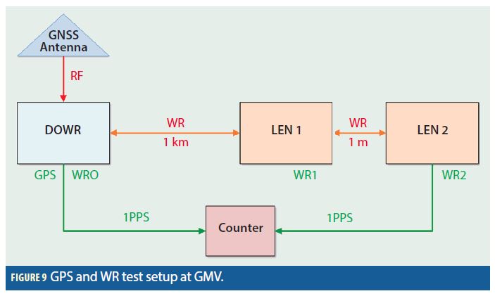
Once the receiver chain has been calibrated, we can input the total delay by configuration in the GPS receiver in order to obtain an output 1PPS signal free of delays. This feature, together with the GPS-to-WR auto-alignment described above, allows the distribution of unbiased timing signals aligned to a known reference (GPSt or UTC) throughout the datacenter. In order to test the time generation and distribution capabilities of GPS combined with WR, we have set up a testing platform at GMV, shown in Figure 8. A schema of the setup is depicted in Figure 9.
In our setup, the timing signals are generated by the newly developed GPS and WR grandmaster (the DOWR), which is connected to a patch GPS antenna on GMV’s rooftop. The receiver is configured to process GPS only, using an accurate fixed position calculated beforehand, and generating a 1PPS aligned to GPSt.
The DOWR is connected in cascade to two WR switches called LENs, using a 1-km optical fiber spool in the first hop, and a 1-m optical fiber segment in the second hop. The DOWR and the LENs provide through a SMA connector the 1PPS generated from WR. The interface between the hardware units and the optical fiber is done through SFP transceivers. A counter is then used to measure the time difference between the original 1PPS from the DOWR and the final 1PPS from the second LEN. The test setup in installed in a standard office, and no particular room temperature control is in place.
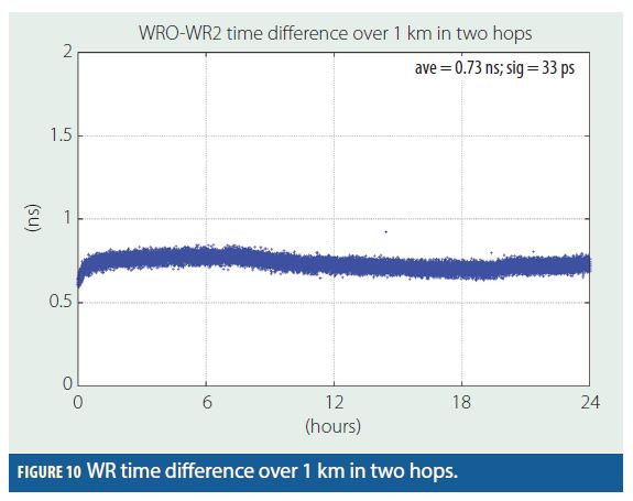
An example of the results over one day can be found in Figure 10, where “WR0” and “WR2” indicate the 1PPS from the DOWR and the 1PPS from the second LEN, respectively. As can be seen, the results show a nearly constant bias of 0.7 ns and an extremely low noise (standard deviation of 33 ps). The slow long-term variation is most likely due to equipment thermal stabilization and temperature variations in the office. The 0.7-ns bias is deterministic and depends mainly on the type and quality of the SFPs, on the number of WR hops, and on the total length of optical fiber.
For a limited number of WR hops (<10) and a limited total length of optical fiber (<10 km), we have observed that the total error in the WR time distribution never exceeds 1 ns. This allows a scalable, sub-ns distribution of timing across multiple servers in the datacenter.
In addition to the WR-derived 1PPS that is distributed downstream, the DOWR outputs through another SMA connector (“AUX”) the native 1PPS signal from GPS. This allows measuring the initial misalignment between the two signals. We have carried out an additional experiment to study the sensitivity of the initial misalignment to power cycles. The DOWR was switched off and on 10 times, and the average offset between its two 1PPS signals (native from GPS and WR-derived) was measured by means of a counter. Notice that a DOWR power cycle implies a complete reacquisition of the GPS signals and a restart of the PVT algorithm. The results show that the GPS-to-WR misalignment fluctuates around zero and is bounded within ± 1 ns, with a resulting standard deviation of 0.5 ns.
Time Traceability and Error Budget
Metrological and legal traceability require an “unbroken chain of calibrations that relate to a reference, with each calibration having a documented measurement uncertainty” (see Matsakis, et alia, Additional Resources). In the field of GPS timing we can consider two well-established references: GPSt and UTC. While GPSt is a real-time time scale available directly from the GPS signals, UTC should be understood as the official UTC maintained by the BIPM, which is only available a posteriori in the Circular T. In the definition of traceability above, “calibration” should be understood in our case as each individual contributor or error source in the whole time generation and distribution chain (i.e., GPS and WR errors).
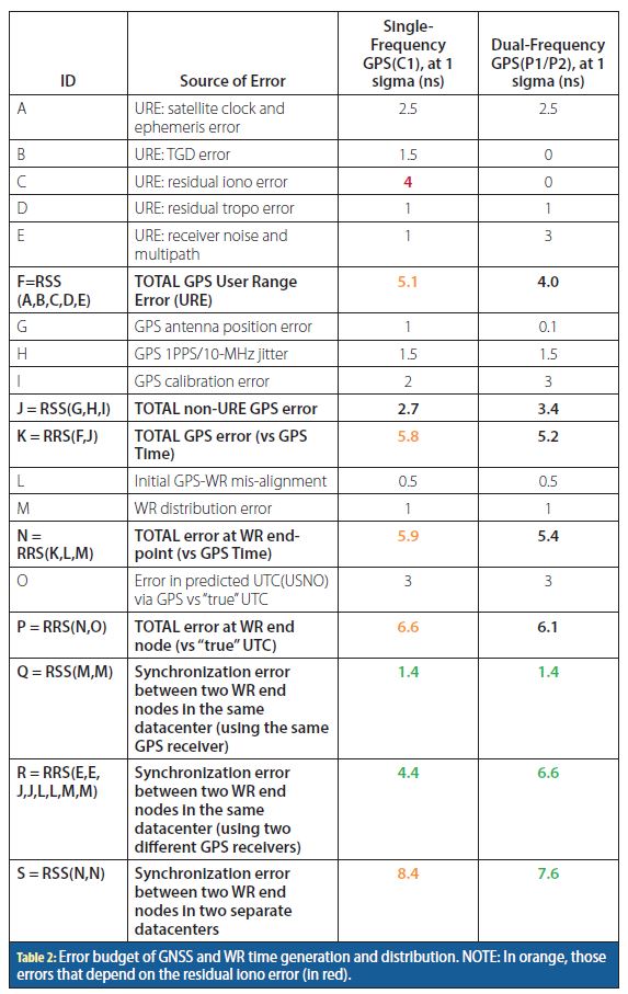
The resulting error budget is shown in Table 2 and is justified in the following paragraphs. Notice that each uncertainty is evaluated at a 1-sigma (68.3%) level of confidence, and that the value generically indicates the combined stochastic (“noise”) and deterministic (“bias”) uncertainty. Constant room temperature is assumed.
For the GPS part, the first factor to consider is whether the receiver is single-frequency (i.e., L1) or dual-frequency (i.e., L1/ L2). Although the DOWR is based on a single-frequency receiver, we develop an error budget for dual-frequency GPS too, for completeness. The main advantage of using dual-frequency GPS is that the ionospheric error in the pseudorange cancels out completely when using the well-known iono-free pseudorange combination. As a downside to this, the receiver noise and multipath error, and to a lesser extent the residual calibration error, are amplified in the GPS iono-free combination.
Our GPS error budget is based on the well-established concept of User Range Error (URE). The URE is the uncertainty in the pseudorange and includes errors from the satellite control segment such as orbit and clock, as well as atmospheric propagation effects, multipath, and user equipment noise. It is reasonable to model these errors as being uncorrelated, and the aggregate URE can be defined as the Root-Sum-Square (RSS) of these individual components. A recent revision of global GPS URE values can be found in the paper by Reid, et alia in Additional Resources. We have adapted slightly these values for our analysis, which is done directly in ns instead of meters. In single-frequency GPS, the residual ionospheric error is the error remaining in the pseudorange after applying the Klobuchar ionospheric model. It is very difficult to give a single value for this error since it depends very strongly on the solar activity, on the time of the day, and on the user location. We have chosen 4 ns as a typical value, as reported by Reid et alia, but this should be taken with caution. The tropospheric error is the error remaining in the pseudorange after applying a recognized model such as MOPS. Regarding the receiver noise and multipath error, we have decided to reduce the value given by Reid et alia (again, see Additional Resources) to 30 cm (i.e., 1 ns), which we believe is more representative of modern receivers, and also in order to cover the possibility of pseudorange smoothing using the carrier. In the case of dual-frequency GPS, we multiply the single-frequency noise and multipath by 3, the iono-free amplification factor in GPS L1/L2.
We have additionally included the contribution of Timing Group Delay (TGD) errors. The broadcast GPS orbits and clocks are computed by the ground control system using the P1/P2 iono-free combination. If the user receiver is single-frequency, the broadcast TGD for each satellite must be added to the broadcast satellite clock in order to align it to the P1 pseudorange. In our error budget we assume a TGD uncertainty of 1.5 ns, which includes possible errors in the broadcast TGDs (see again Garbin, et alia) and also a possible lack of knowledge about the C1-P1 satellite bias (which is only broadcast in the new CNAV message of GPS).
In GPS positioning, the user position error is the combination of several factors, namely, the URE, the number of satellites in view, and the user-satellite geometry. The case of GPS timing is somewhat different since most timing receivers allow to “fix” the antenna position to a pre-computed value, and thus a minimum of just one satellite is required to estimate the receiver clock bias. For simplicity, in our error budget calculation we will assume a “minimum timing scenario” with fixed position and only one GPS satellite in view, thus the URE projects directly into a time error. In this scenario there is no degradation in the time error due to position calculation, but there is also no improvement in the time error from the usage of several satellites. We assume an antenna 3D position error of 30 cm (1 ns) in single-frequency and 3 cm (0.1 ns) in dual-frequency. This position accuracy can be obtained offline using for example Precise Point Positioning (PPP) processing a raw measurement batch of 1-day duration. Also, we will assume that the instantaneous error in the receiver clock bias estimation from GPS translates directly into a 1PPS error, although this could be smoothed out using a stable receiver clock and a suitable steering algorithm.
Additional effects associated to the GPS receiver are taken into account such as a possible jitter on its output 1PPS (1.5 ns), and a residual error in the GPS calibration: 2.0 ns in single-frequency (C1), and 3.0 ns in dual-frequency (P1/P2). For the WR part, we include the initial misalignment between the GPS and WR 1PPS signals, and the time distribution error along a typical WR chain (0.5 ns and 1 ns, respectively, as explained in the previous section).
The error in the UTC distributed by GPS in its navigation message is considered as the last contribution, so that we can analyze separately the case when the user selects GPSt as a reference and the case when UTC is used. The UTC error is actually composed of two parts: the first part is derived from the fact that the UTC realization used by GPS, i.e., UTC(USNO), actually deviates from the official UTC published by the BIPM; the second part is due to the prediction error of UTC(USNO) relative to GPSt, as contained in the GPS navigation message. We estimate the combined UTC uncertainty to be 3 ns.
All the errors described above can be considered as uncorrelated, so the aggregate total error can be calculated as the RSS of the individual error sources. As a result, we obtain the total time error at the WR end node, using a single-frequency or a dual-frequency GPS receiver, and using GPSt or UTC as reference (see rows N and P in Table 2).
It is also of interest to estimate the relative synchronization error between two WR end nodes in the same datacenter. If a single GPS receiver is used for the whole datacenter, only the WR distribution error must be considered (row Q). If different receivers are used in the datacenter, all URE errors, except the intrinsic receiver noise and multipath, can be considered very similar (because of the same geographical location) and cancel out between receivers, and only noise and multipath, non-URE GPS errors, and WR-related errors must be considered (row R).
Finally, we can estimate the relative synchronization error between two WR end nodes in two separate datacenters located anywhere in the world (row S). In this case we can consider all the errors described above as uncorrelated between the two sites, except the UTC error, which is common to all sites, since the predicted offset of UTC to GPSt is a global model transmitted by the constellation. When using UTC as reference, the UTC error cancels out between the two sites, thus the synchronization error between the two sites is the same one as when using GPSt as reference.
In all cases (intra-datacenter and inter-datacenter) we assume that the same type of receiver (single-frequency or dual-frequency) and the same time reference (GPSt or UTC) is used everywhere.
Conclusions
By accurately calibrating the GPS receiver chain and seamlessly integrating the GPS and White Rabbit timing signals, we are able to distribute the timing from GPS via WR with a degradation of just around 1 ns over 1 km. Using single-frequency GPS, and considering all GPS and WR errors, we are able to timestamp (and therefore synchronize) any server inside a datacenter with a typical error smaller than 10 ns (at 1 sigma) versus UTC. Furthermore, given the ubiquity of GPS, the approach can be applied to datacenters at any location in the world. Assuming uncorrelated errors between separate sites, we can establish that any pair of servers in the world can be synchronized to each other with a typical error also smaller than 10 ns (at 1 sigma). This is particularly interesting to guarantee the consistency and transaction ordering of distributed databases and financial trading engines.
The usage of dual-frequency GPS for timing is not extremely advantageous. The ionospheric error cancels out completely using dual-frequency, but the receiver noise and multipath error gets amplified by a factor of 3 in the iono-free combination. Also, the residual GPS calibration error is roughly doubled in the iono-free combination, depending on the calibration technique employed. In consequence, in moderate solar activity the typical single-frequency timing uncertainty is only slightly larger than the dual-frequency one. This conclusion should be taken with caution since the instantaneous ionospheric error could be much larger depending on the solar activity, on the time of the day, and on the user location.
Manufacturers
The golden GNSS receiver chain absolutely calibrated is composed of a multi-frequency Septentrio PolaRx5TR time-transfer receiver, and a multi-band Leica AR20 choke-ring geodetic-type antenna.
The LEN is a WR switch and end node developed by Seven Solutions. The DOWR is a new GPS and WR grandmaster device developed jointly by Seven Solutions and GMV, based on the LEN platform.
The DOWR and the two receiver chains calibrated at PTB in 2017 incorporate the single-frequency (L1) LEA-M8F receiver from u-blox, connected to a single-band Tallysman TW2710 patch antenna.
The time interval counter used at GMV is a Keysight 53230A providing 20-ps resolution.
Additional Resources:
1. Garbin, E., P. Defraigne, P. Krystek, R. Píriz, B. Bertrand, P. Waller, “Absolute calibration of GNSS timing stations and its applicability to real signals”, Metrologia, Volume 56, Number 1, 14 December 2018
2. Matsakis, D., J. Levine, M. Lombardi, “Metrological and Legal Traceability of Time Signals”, Proceedings of the 49th Annual Precise Time and Time Interval Systems and Applications Meeting, Reston, Virginia, January 2018, pp. 59-71
3. Reid, T. G. R. , A. M. Neish, T. Walter, P.K. Enge, “Broadband LEO Constellations for Navigation”, J Inst Navig, 65: 205–220, 2018
4. Serrano, J., M. Cattin, E. Gousiou, E. van der Bij, T. Włostowski, G. Daniluk, M. Lipinski,, “The White Rabbit Project”, IBIC 2013
Authors
Ricardo Píriz is an aeronautical engineer from the Polytechnic University of Madrid. He started his career as a Flight Dynamics engineer in the Precise Orbit Determination group at ESOC, the European Space Operations Center in Darmstadt, Germany. Later on he moved to Eutelsat in Paris, as a Mission Analysis engineer in the Satellite Procurement Division. Since 2001 he has been in the GNSS Business Unit of GMV working on several projects, in particular in the GIOVE Mission (the experimental phase of Galileo), and in the Galileo Time Validation Facility (TVF). He is currently Leader of the GNSS Time & Frequency Group.
Esteban Garbin is an Electronics and Telecommunication engineer who got his Ph. D. from Politecnico di Torino in 2017. His research studies focused mainly on GNSS receivers and signal processing algorithms, particularly for interference and spoofing detection and mitigation. Since June 2017 he has been working for GMV, focusing on different aspects in the GNSS Advanced User Segment solutions division, mainly developing novel concepts on GNSS timing and receivers.
Javier Díaz received the M.S. degree in electronics engineering and the Ph. D. degree in electronics from the University of Granada, Spain, in 2002 and 2006, respectively. He is currently an Associate Professor with the Department of Computer Architecture and Technology, University of Granada. His current interests include high-performance image processing architectures, safety-critical systems, highly accurate time synchronization, and frequency distribution techniques. He is also co-founder of Seven Solutions, a leading company in White Rabbit technology based in Granada, Spain.
Pascale Defraigne is Project Leader at the Royal Observatory of Belgium. She completed her PhD in Physics at the Université Catholique de Louvain (UCL), Belgium, in 1995, for studies on mantle convection and deformations of the Earth internal boundaries. She then moved to the Royal Observatory of Belgium to start research activities on GNSS time and frequency transfer. Her research activities include remote atomic clock comparisons, time scale generation, and ionospheric sounding based on GNSS measurements. She is deeply involved in the development and upgrade of the Galileo System for all what concerns the Galileo System Time. Among her involvement in international bodies, she assured the Presidency of the Commission 31 “TIME” of the International Astronomical Union (2006-2009) and since 2012 assures the Chair of the CCTF Working Group on GNSS Time Transfer (CCTF being the Consultative Committee for Time and Frequency, sub-committee of the International Committee for Weights and Measurements). She also is a member of the GNSS Science Advisory Committee of the European Space Agency since 2012.


