Scintillation — rapid RF signal frequency and amplitude changes due to signal propagation path changes and phase shifting caused by solar turbulence in the ionosphere — is well known in the GNSS community. However, conclusive scientific studies that cover the whole extent of the question are hard to find. Galileo In-Orbit Validation Experiment (GIOVE) data processing confirmed the effects of scintillation on GNSS receivers, as described in the paper by J. Giraud listed in the Additional Resources section near the end of this article.
Scintillation — rapid RF signal frequency and amplitude changes due to signal propagation path changes and phase shifting caused by solar turbulence in the ionosphere — is well known in the GNSS community. However, conclusive scientific studies that cover the whole extent of the question are hard to find. Galileo In-Orbit Validation Experiment (GIOVE) data processing confirmed the effects of scintillation on GNSS receivers, as described in the paper by J. Giraud listed in the Additional Resources section near the end of this article.
For example, the fading due to the ionosphere scintillation observed at the Galileo station in the Guiana Space Center (CSG), near Kourou, French Guiana, shows an amplitude of more than 10 decibels. The measured carrier phase jitter also demonstrated potential issues on tracking loop stability, which could have an impact on the station’s receiver availability and/or design and, of course, have an impact on the user receiver behavior.
As far as Africa is concerned, the lack of GNSS stations in the sub-Saharan region exacerbates the difficulties of investigating the ionospheric effects on GNSS signal propagation. This situation triggered the joint initiative of the French space agency CNES (Centre National d’Etudes Spatiales), the Agency for Air Navigation safety in Africa and Madagascar ASECNA (Agence pour la Sécurité de la Navigation Aérienne en Afrique et à Madagascar), and Thales Alenia Space to deploy a reliable network of stations, with the goal of providing an efficient tool for scientific developments on the particular issue of ionosphere.
This article describes the network itself as well as early preliminary observations.
Based on observations made during the first six months of exploitation, some analyses were made on the modeling of the ionosphere at those latitudes, with particular attention paid to the strong gradient that can be encountered. For this, we analyzed several models’ accuracy over a small period of observation. Further observations are now about to be implemented for long-period accuracy analysis.
SAGAIE : The Network of Stations
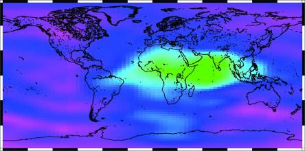
CNES and ASECNA, with the support of Thales Alenia Space, jointly deployed a network of GNSS sensors covering the Western Africa Region (see Figure 1) known as SAGAIE (Stations ASECNA GNSS pour l’Analyse de la Ionosphère Equatoriale, or GNSS ASECNA Stations for the Analysis of the Equatorial Ionosphere). The stations are all installed at major airports of the region: Dakar, Lomé, Ouagadougou, Douala, and N’Djamena. These sites also match with maximum ionosphere activity as illustrated in Figure 2.
Choosing airport sites for deployment ensures that the operations of the stations can benefit from the infrastructures of ASECNA already in place. In particular, these sites provide high-stability power supply and reliable Internet access to make measurements widely available in near–real time with high stability. Airport installations also ensure a stable temperature for the receivers, as they are all installed in rooms with air conditioning.
The stations employ three different types of receivers: a GPS/GLONASS/Galileo multi-frequency ionospheric scintillation monitor, an enclosure containing a triple-frequency plus L-band GNSS receiver board, and one multi-channel, multi-constellation environmental monitoring software GNSS receiver. Two sites are equipped with the full set of receivers, Dakar and Lomé. The Ouagadougou, Douala, and N’Djamena sites use the GNSS receiver enclosure only.
GNSS antennas greatly affect the quality of the measurements. Two stations (Dakar and Lomé) are equipped with choke ring antennas, whereas Douala, Ouagadougou, and N’Djamena are equipped with triple-frequency “pinwheel” antennas.
All receivers are compatible with the following signals:
- GPS L1 C/A, L2C, L5 and L1/2P semi codeless,
- Galileo E1, E5a/b
- Glonass G1, G2
- SBAS L1/L5
The receivers provide unfiltered measurements on all frequencies.
SAGAIE stations are also equipped with two universal software radio peripheral (USRP) boards in order to sample the RF dual-frequency signal and process it with the software receiver as well as storing it for further analyses when high scintillation is detected. Figure 3 shows the equipment configuration at the SAGAIE stations.
The GNSS observations (sampled at one hertz) from the receivers are stored locally as Receiver-INdependent EXchange (RINEX 3) and ISM files and forwarded to a central server at CNES in Toulouse for further processing and archiving. Figure 4 provides a schematic of the SAGAIE network architecture. The data transfer is made every 15 minutes for nearly real-time analysis. The local storage makes the station robust to any temporary loss of an Internet connection.
In parallel to the 15-minute transfer process, a real-time NTRIP (Network Transport of RTCM via Internet Protocol) process transfers the differentially corrected data to the CNES Internet caster for real-time distribution. Contrary to the 15-minute transfer process, this NTRIP transfer is not robust against Internet losses and might incur some data loss.
The stations’ software receivers are designed around graphics processing unit (GPU)-based fast processing and controlled locally and remotely by a survey software suite. This software suite controls the local data archiving, the data transfers without loss, and any type of commands sent to the receiver by the administrators.
Coupled with the software receiver, the software suite allows the storing of raw sampled dual-frequency signals when a scintillation is detected. This mechanism enables us to capture pieces of strongly disturbed signals for a posteriori analyses. The flexibility of the software receiver associated with a fast replay mode allows for remote testing of new algorithms to compare performance on a strongly affected signal for receiver-specific research.
High RF Quality and Signal Availability of Sites
Selection of SAGAIE station deployment was based on a site survey phase. Particular attention was paid to select sites where local propagation effects (multipath and interference) would be minimized. Most antennas are situated on top of control towers with a clear sky view as shown in Figure 5 for Ouagadougou and Figure 6 for Douala.
After six months of data gathering, we compared the quality of the SAGAIE sites with those of the International GNSS Service (IGS), in particular regarding multipath. Figure 7 presents a comparison of SAGAIE multipath errors based on GPS dual-frequency measurements with those of all IGS stations as available here. It turns out that the SAGAIE stations and sites are comparable and could even be among the best of the IGS facilities.
As far as data availability is concerned, the survey software administration web tool provides an example of 100 percent availability over a period of one month for Ouagadougou’s station (Figure 8).
Internet-Based Survey Software
Let’s look a little more closely at the Internet-based survey software suite through which the SAGAIE network is remotely controlled. As mentioned earlier, it supports real-time control of the behavior of the stations, data archiving, and remote placing of commands to the receivers in a unified interface for all the receiver types deployed at the SAGAIE stations. Figure 9 shows the command and control screen for this software.
Besides the application dedicated to real-time interfacing with the deployed stations, the survey software suite also comprises web services that allow, on the one hand, monitoring of transfers and quality of data and on the other hand produces daily and monthly analyses of the data, as shown in Figure 10, Figure 11, and Figure 12.
A Remotely Controlled Software Receiver
The GNSS environmental monitoring receiver is a full software-based solution developed to assess the quality of GNSS measurements. It is composed of a signal-processing module called GEA (GNSS Environment Analyzer) that features error identification and characterization functions, integrated with the survey software suite as a complete graphical user interface and database management system.
The GEA module lies at the heart of the software receiver. This module contains the entire signal-processing functions required to build all the GNSS observables that are often used for signal quality monitoring (SQM). A C/C++ software based on innovative GPU parallel computing, the GEA module enables the processing of large quantities of data very quickly. It can operate seamlessly on a desktop or a laptop while adjusting its processing capabilities to the processing power available on the platform on which it is installed.
The signal-processing module of GEA can handle multiple channels and constellations, and supports both real-time and post-processing of GNSS samples produced by an RF front-end. Its CPU-based and GPU-based correlation engines (for both acquisition and tracking) are accessed through its open application programming interface (API), allowing the implementation of third-party algorithms for specific analyses or R&D studies that would not be possible with the default-embedded GEA algorithms.
Being entirely software, GEA is easily integrated with other elements, such as system performance tools, or used to emulate different classes of GNSS receivers. The GEA module also has embedded SQM algorithms aimed at characterizing reception conditions, with a specific focus on interference, ionosphere scintillation, multipath, and “evil” waveforms.
Figure 13 shows the software architecture of GEA. As of today, the GEA module supports GPS L1C/A, L2C, and L5; Galileo E1OS, E5a, and E5b; GLONASS G1 and G2; BeiDou B1I and B2I; and space-based augmentation system (SBAS) frequencies L1 and L5.
A software client is integrated with GEA to manage the connections and the requests to an assistance server following 3GPP standards. Another particularly interesting assistance methodology supported by GEA is the National Geodetic Survey’s orbital format sp3 (StandardProduct # 3). This mode is employed to analyze the accuracy of the measurements using the high-accuracy sp3 orbits available from the IGS. In such cases, the reference location is provided through a scenario configuration file and precise timing synchronization is done using the GEA RF front-end trigger connected to the constellation simulator and 10-megahertz inputs.
SAGAIE takes advantage of the software receiver’s flexibility to analyze the performance of several receiver configurations and algorithms in the presence of strong scintillation. The fast processing capabilities of software receiver allows for very quick replay and paves the way for testing of a large number of algorithms on locally stored signal snapshots.
Based on an Nvidia graphical card, GEA is able to process many signals in parallel, on top of which analysis modules are run. The number of correlators and their relative placement is fully configurable through the GEA configuration file, which eases the development of innovative algorithms.
Note that the GEA architecture is ready to accommodate larger sampling frequencies by simply increasing the number of GPU cards to maintain the real time capabilities of the software. Such a configuration is typically used within TAS-F and CNES to process the signal at 137 megahertz in real time.
The software receiver’s command and control is accomplished through the man/machine interface (MMI) and the Internet-based survey software that controls all the receivers in the SAGAIE stations. When controlling the software receiver, the MMI displays in real time the three-dimensional autocorrelation function of the processed signals, as well as the -dimensional “waterfall” view (seen in the left hand-side of Figure 14), in which multipath and ionosphere scintillation effects can clearly be observed. The software receiver can display a large variety of observables on the monitor screen. In addition to the visualization of GEA outputs, the interface of the software receiver allows for data storage and display in a database of measurements and analysis results.
SAGAIE Products
The SAGAIE web environment realizes daily statistics on the scintillation activity over all the SAGAIE stations. This allows us to gather a backload of information in order to establish reliable statistics on the real scintillation phenomenon in Africa.
Quasi–Real-Time Ionosphere Models. Despite the mere observation of the GNSS amplitude scintillation index (S4) and the phase scintillation index (σφ), one of the missions of the SAGAIE network is to evaluate the relevance of various ionosphere models in regions like the sub-Saharan. For this, the SAGAIE information system (maintained through the Internet-based survey software) is about to be upgraded to supply several ionosphere models, which can be fitted every five minutes for the subsequent five minutes. The goal is to evaluate the performance of several models.
To model the ionosphere (or more exactly the electron density), one solution is to represent the ionosphere as a simple thin shell model (Figure 16). To compute the ionospheric pierce point (IPP), we need to know the receiver and satellite position, and the altitude of the thin shell layer (see RTCA, Inc., MOPS 229 in Additional Resources). Usually, we assume an altitude of 350 kilometers in order to represent the F layer that contains the electron density peak.
However, the estimated total electron content (TEC) is by definition an integrated observable. Thus, the TEC estimated at an IPP will depend on the ionosphere thickness or, in other words, on the path elevation. In order to have an independent measurement of the elevation, the vertical TEC (denoted TECv) is commonly used. A slant factor is links the TEC and the TECv (as discussed in the RTCA MOPS 229).
The SAGAIE system provides several ionospheric models whose coefficients are fitted out of the real station measurements: Klobuchar, Taylor, Spherical Harmonic, and NeQuick.
The most popular model is the Klobuchar model, which represents the ionospheric delay as a sinusoid function of time. The amplitude and the period of the sinusoid can be tuned as a function of the IPP position thanks to eight parameters.
Based on dual-frequency measurements, we can invert the Klobuchar model in order to update the Klobuchar coefficients with a predefined rate. The SAGAIE server provides results of the estimation for local Klobuchar as compared to the Global GPS-broadcast model. In the following discussion, the SAGAIE Klobuchar product fitted onto the SAGAIE measurements is identified as the “updated Klobuchar model.”
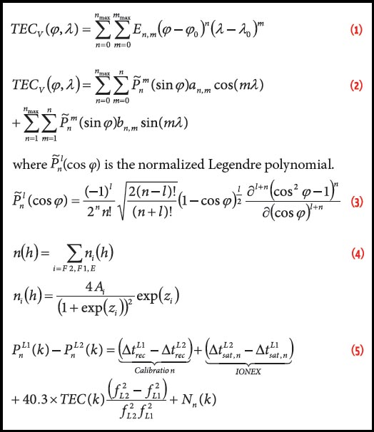
The Taylor model represents the evolution in space of the TECv as a Taylor expansion around a reference latitude and longitude (λ0, φ0). The TECv is given by Eq. (1):
Equation (1) (See inset photo, Above right, for all equations)
where (λ, φ) are respectively the latitude and the longitude of the IPP, (nmax, mmax) are the order of the Taylor development, respectively, on the φ and λ dimensions, and En,m are the Taylor parameters. For the time being, the SAGAIE system considers the same order for both dimensions, nmax = mmax. The Taylor coefficients are estimated with a least mean squares algorithm based on dual frequency information provided by the SAGAIE receivers.
The spherical harmonic model represents the TECv by a combination of the Legendre polynomial Eq. (2).
Equation (2)
Equation (3)
As in the Taylor expansion, the SAGAIE system uses a least mean square estimation based on dual-frequency information in order to estimate the spherical harmonic coefficients (an,m, bn,m).
The NeQuick model abandons the supposition of a thin shell surface, along with the necessity of projecting a “vertical effect” through a slanting function. The NeQuick model provides a four-dimensional representation (space and time) of the electron density (n0). It is a semi-empirical model in the sense that the model takes into account the physical properties of the various ionospheric regions. In the NeQuick model, the ionosphere is vertically divided into three parts: E, F1, and F2 regions. Each region uses a sum of Epstein layers (discussed in the articles by S. M. Radicella et alia and Y. Memarzadeh cited in Additional Resources): the formulation is such that the model and its first derivative are always continuous.
Equation (4)
The parameters Ai and zi model the electron maximum and the thickness of each layer. These parameters depend on the modeled layer — the paper by Y. Memarzadeh summarizes these quantities for each layer — and also on the ionosonde parameters, which are foE, foF1, foF2, and M(3000)F2. These parameters are calculated using four inputs: the dip latitude, the receiver position, the solar activity level (F10.7), and the coordinated universal time (UTC). Figure 17 summarizes the NeQuick principle.
To compute the ionosonde parameters of the F2 region (i.e., foF2 and (3000)F2), NeQuick was originally developed to use the monthly averaged F10.7 index of solar activity. To use the NeQuick model for real-time applications, such as a Galileo ionospheric correction model, the monthly averaged F10.7 index is replaced by a daily input parameter to take into account the daily variation of the solar activity and the user’s local geomagnetic conditions. This daily NeQuick input parameter is the so-called effective ionization level, which is denoted by Az in units of solar flux, 10−22 Wm−2 Hz−1. It characterizes the physical conditions of the ionosphere.
The Az parameter is computed by a second order polynomial, where the three coefficients are, for instance, broadcast in the Galileo navigation message. Finally, the main inputs of the NeQuick model are the receiver position, the satellite position, the time (year, month, day, UTC time), and the solar flux (or ionization level parameter). (See Additional Resources for sources of average solar flux and NeQuick parameters.)
Some Statistics on Ionosphere. From the deployment onward (10 months for some stations), 12 terabytes of data have been accumulated. In addition to some very specific analyses of the scintillation phenomena, statistical analyses have been carried out, especially to quantify the phenomenon. We provide here a sample of the outputs for two stations, Dakar and Lomé. Figure 18 provides the number of scintillations events (S4>0.5) detected each month to illustrate its seasonal aspects close to the equinoxes. Figure 19 provides the repartition of these events along the elevation of the satellites. Signals coming from satellites at low elevation angles are much more affected than those at higher elevation angles.
Finally, Figure 20 compares the repartition of the scintillations versus the number of satellite/receiver lines of sight that are impacted, taking into account that GPS, GLONASS, and Galileo satellites are being tracked. Those statistics are generated directly in the multi-frequency ionospheric scintillation monitor receiver outputs.
Interfrequency Bias: A Key Issue for Ionosphere Measurements
To evaluate the ionospheric delay, the standard method consists of comparing the pseudoranges between L1 and L2 bands such as in Eq. (5):
Equation (5)
where PnLi(k) denotes the pseudorange for the Li band, Δtrec is the receiver clock bias, Δtsat is the satellite clock bias, TEC(k) is the TEC that represents the integration of the electron density along the path, fLi is the carrier frequency, N is the noise combination between both bands, and n represents the satellite index.
In order to evaluate the ionospheric delay (or, in other words, the TEC), we needed to remove the interfrequency bias at the receiver and satellite stage. SAGAIE automatically implements two processes. First, a calibration is made in the lab using a controlled signal generator developed by CNES and Thales Alenia Space, Navys. Second, a calibration process is implemented each day, assuming that the interfrequency bias is constant during the day.
In order to improve the estimation accuracy, the process implements a code-carrier smoothing. Figure 21 and Figure 22, respectively, represent the estimated ionospheric delay as a function of time for the Dakar station and as a function of space for the Douala station. Figure 21 represents the delay as a function of IPP associated with a thin layer at 350 kilometers.
Comparison of Ionospheric Models
Based on initial results supplied by the SAGAIE system, we evaluated and compared the performance of each model, taking into account three criteria:
- mean estimation error of the delay
- time validity of the models
- coverage of the models.
The following are very preliminary results, as they result from only a few days of examination.
To evaluate the first two criteria, we tuned the SAGAIE system so that every five minutes the coefficients of the models are estimated based on the accumulation of five minutes of data at one hertz. After creation of the model, we observed the error associated with the propagation of the model over time, which provides information about the validity period of the model.
Figure 23 presents an example of the results of this technique. The figure displays the mean absolute error associated with the updated Klobuchar model and with a second-order Taylor model when these models are created at t = 3h45, 6h45, and 14h45. This figure also plots the error of the GPS-broadcast Klobuchar model and the error associated with the IONosphere EXchange format (IONEX). The mean ionospheric delay observed through dual-frequency measurements is also displayed.
As one can see, after the models’ creation, the models based on data fitting provide the same mean error during a short time period, typically 12 minutes, as a worst case for the Taylor Third Order. After a relatively stable period of validity, the model rendering error degrades rapidly.
We also report a sampling over five non-consecutive days (08/28/2013, 09/07/2013, 10/02/2013, 11/27/2013, 12/16/2013) in Table 1, giving the mean ionospheric error and the minimum updating period of the model coefficients.
The SAGAIE system compares the IONEX TECv map with the TECv map provided by estimates from the SAGAIE internal models. Figure 24, Figure 25, and Figure 26 present the absolute difference between the IONEX map (in meters on L1) and several ionospheric models that are part of the SAGAIE products. These examples were generated on September 17, 2013, at around 14:00 UTC.
Figure 24 illustrates how local estimation of the Klobuchar model provides better results for local applicability. The mean estimated coverage associated with each model for all the processed days are presented in Table 1.
Based on the results of this first exploitation period, which is very limited in time, we anticipate that higher-order Taylor models provide the best representation of the ionosphere in the sub-Saharan region and that the NeQuick model provides the best forecasting capability.
Obviously, we can note that the higher the order of the model, the better the ionospheric delay estimation, but the smaller the period of validity. For a given order, the spherical harmonic and Taylor models provide approximately the same performance.
Single-Station Assessment of Model Performance
The SAGAIE system allows us to build models thanks to the data taken from four stations (Dakar, Lomé, Douala, and N’Djamena), and to evaluate the model errors using data from another station (Ouagadougou, not used in the inverse problem). Figure 27 and Figure 28 both represent the average ionospheric model error (over all visible satellites) of the Taylor and spherical harmonic models in Ouagadougou, when using data from the four other stations to estimate the model parameters.
The actual ionospheric delay is estimated through dual-frequency measurements made with the Ouagadougou receiver. This enables us to estimate the error of the model over Ouagadougou. As we can see, the performance in term of ionospheric delay estimation provided by the real-time SAGAIE-estimated models is very good and close to the IONEX model.
Scintillation Impacts on Ionosphere Model Estimation
As a baseline, the estimation process refreshes the model coefficients every 300 seconds for a validity period extending over the next 300 seconds. With this principle, we analyzed the result of the successive estimations over an analysis period of seven days, of which two days were polluted by strong scintillation events (02/17/2014 and 03/02/2014). A scintillation example is given in Figure 29 that illustrates the high jitter on the C/N0 appearing on the estimation at t = 20 hours and t = 21 hours 15 minutes. For these two events, we note that the ionospheric delay is suddenly decreasing, which must be due to the presence of plasma bubbles.
Figure 30 and Figure 31 present, respectively, the models’ absolute mean error (over all visible satellites) for one day without scintillation (08/28/2013) and one day with scintillation (02/17/2014). Table 2 summarizes the results in terms of mean error and standard deviation for all the processed days. In these figures and table, we present the performance of the SAGAIE model, with a sub-sampled grid in order to fit with the traditional SBAS grid (5°x5°). This is referred to as “SBAS-like.”
From these results, we can observe that in these scintillation conditions the performance of the model is quite conservative for low-order models. However, for higher order models, our experience indicates that the maximum error can be important.
What’s Next?
The SAGAIE network is now operational. Several automatic tools have been deployed as reflected in these initial results. This will allow us to accumulate information regarding the ionospheric conditions in sub-Saharan regions. With the tools in place, CNES and ASECNA need to step back in order to accumulate statistical data on the ionosphere conditions in the region. Moreover, the SAGAIE network may also grow into a denser geographic footprint.
Regarding the acquired signals, a very large amount of data has been collected (more than 12 terabytes). They will soon be used to analyze the behavior of the receiver under scintillation and to further test robust algorithms that enable the receiver to remain locked on the signal, especially considering the use of new Galileo signals supplying with pilot tones. The recorded raw signals could also be used as a basis for RF replay in order to test real aeronautical receivers behavior. The interaction with the ionosphere model estimation will also be analyzed.
Conclusions
This article has described the SAGAIE GNSS sensor station network. The very early exploitation phase allowed primary analyses of model performance over sub-Saharan regions. It also allowed analyzing the strength of the scintillation over the region in the past 6–10 months.
Some preliminary observations have been made, such as the performance of the ionosphere models in the regions, but these preliminary results are based on a very short exploitation period and need to be accumulated over a more extended period of time. The SAGAIE network is now in place and paves the way for very interesting results that should come soon.
In the meantime, the MONITOR project has been launched by ESA to analyze the ionosphere’s behavior in low and high latitudes. Both MONITOR and SAGAIE stations will contribute to a better understanding of the ionosphere’s impact on GNSS.
Acknowledgments
The authors thank ASECNA for their support to maintain the network in good operational conditions. In particular, Roland Kameni, SAGAIE responsible at ASECNA; Herbert N’Gaya without whom the deployment would not have been so easy; Yao Anoba (responsible for Lomé’s Station), Michel Tagnan (responsible for Ouagadougou’s station), Joachim Molina (responsible for Douala’s station), Severine Diongoussou (responsible for N’Djamena’s station), and Haroun Mahamat (responsible for Dakar).
Additional Resources
[1] Average solar flux F10.7 is available here
[2] Di Giovanni, G., and S. M. Radicella, “An Analytical Model of the Electron Density Profile in the Ionosphere,” Advances in Space Research, Vol. 10, No. 11, pp. 27-30, 1990
[3] Giraud, J., “Latest Achievements in GIOVE Signal and Sensor Station Experimentations,” ION 2009
[4] Klobuchar, J., “Ionospheric Time-Delay Algorithms for Single-Frequency GPS User,” IEEE Transactions on Aerospace and Electronic Systems, pp. 325-331, 1987
[5] Memarzadeh, Y., Ionospheric Modeling for Precise GNSS Application, PhD dissertation, December 2009
[6] NeQuick broadcast parameters are available here
[7] Parkinson, B. W., and J. J. Spilker, Global Positioning System: Theory and Application, Volume 1, Progress in Astronautics and Aeronautics, Volume 163, 1996
[8] Radicella, S. M., and M. L. Zhang, The Improved DGR Analytical Model of Electron Density Height Profile and Total Electron Content in the Ionosphere, Annali di Geofisica, pp. 35-41, 1995
[9] RTCA Inc., DO-229B Minimum Operational Performance Standards for Global Positioning System/Wide Area Augmentation System Airborne Equipment
[10] Van Dierendonck, A. J., and B. Arbesser-Rastburg, Measuring Ionospheric Scintillation in the Equatorial Region over Africa, including Measurements from SBAS Geostationary Satellite Signals
