Errors in inertial sensor measurements are accumulated over time, leading to drift in INS navigation outputs. While gyro bias is the main contributor, other factors, such as accelerometer bias and noise, are important to consider for balancing the overall error budget.
A key benefit of inertial navigation is its self-contained nature as the system can maintain navigation continuity while other navigation aids are (temporarily) unavailable. For example, GNSS/INS mechanization can coast on inertial solution when GNSS is jammed. Yet, as described in the previous column on inertial fundamentals, integration is the main computational operation of the INS: sensor measurements (angular rates and non-gravitational acceleration components also referred to as specific forces) are integrated into navigation outputs (attitude, velocity and position). Measurement errors are integrated as well, which leads to a drift in navigation solution over time. As a result, inertial can be used to bridge over continuity gaps (such as GNSS interference areas), but over a limited time.
Understanding inertial error behavior is a critical component of the overall system design. It is addressed in this column.
Influence of Accelerometer Bias
We start with a simple one-dimensional (1D) case where a platform moves along the x-axis of the horizontal frame. In this case, the double integration scheme completely defines the INS navigation mechanization because attitude determination, gravity addition and coordinate transformation are not required. A constant bias, baccel, in accelerometer measurements propagates into velocity and position errors (δv and δr, respectively) as follows:


Influence of Gyro Bias
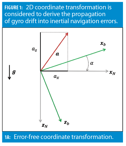
Gyro bias is first integrated into attitude errors and then propagates into velocity and position errors through coordinate transformation. To understand the error propagation mechanism, let’s consider a simplified two-dimensional (2D) case that is illustrated in Figure 1.
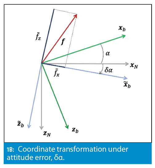
In Figure 1(a) the relative angle, α, between the body-frame (xb, zb) and the navigation frame (xN, zN) is perfectly known. In this case, body-frame non-gravitational acceleration is translated exactly into its navigation frame components, ax and az. When gyro bias, bgyro, is present, it is integrated into the attitude error, δα, during the attitude determination step:

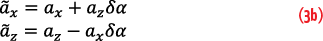
where δα is the initial attitude error. As a result, instead of being computationally aligned with the actual navigation frame, the body-frame is rotated into a tilted frame as shown in Figure 2 (b). In this case, the non-gravitational acceleration transforms as:
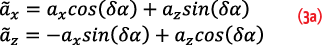
or using the small angle approximations (i.e., cos(δα)≈1 and sin(δα)≈δα):
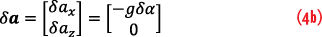
Hence, the error in the coordinate transformation, δα, leads to acceleration-domain errors, azδα and -axδα, that are then double integrated into position error. This leads to cubic growth of position error due to gyro bias. To illustrate, consider a stationary case where:

In this case, the coordinate transformation error, δa, is:
When integrated into position error, it becomes:

For a general 3D case, the consideration is substantially more involved mathematically. Yet, the nature of error propagation remains the same: gyro bias-induced position error growths proportionally to time3.
The Shuler Effect
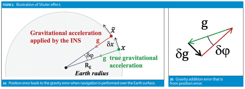
These considerations show accelerometer and gyro drift lead to unlimited error growth in INS navigation outputs. However, when navigating over the Earth surface, the horizontal error component becomes limited due to a Shuler effect. This effect introduces negative feedback (via the gravity addition step) into the error propagation mechanism, thus transforming the polynomial error growth into an oscillatory behavior. The oscillation period is rather large (about 84 minutes as we will see later in this section). As a result, it does not have much benefit for lower-grade inertial systems as their errors grow to unacceptable levels before the Shuler effect kicks in. Yet, Shuler oscillations effectively limit horizontal errors of a high-quality system such as a navigation-grade INS. Figure 2 illustrates the Shuler effect.
As shown in Figure 2, position error δx leads to the wrong gravitational acceleration vector being applied for the gravity addition step. This creates an acceleration error:

Because the acceleration error is the second derivative of the position error , Equation 5 can be rewritten as:
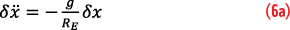

Equation 6 is a well-known differential equation of a harmonic oscillator. Thus, the position error has an oscillatory behavior with its (Shuler) oscillation period, TS, defined as:
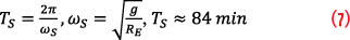
Table 1 shows the INS error propagation mechanism for different error sources when the Shuler effect is taken into account.
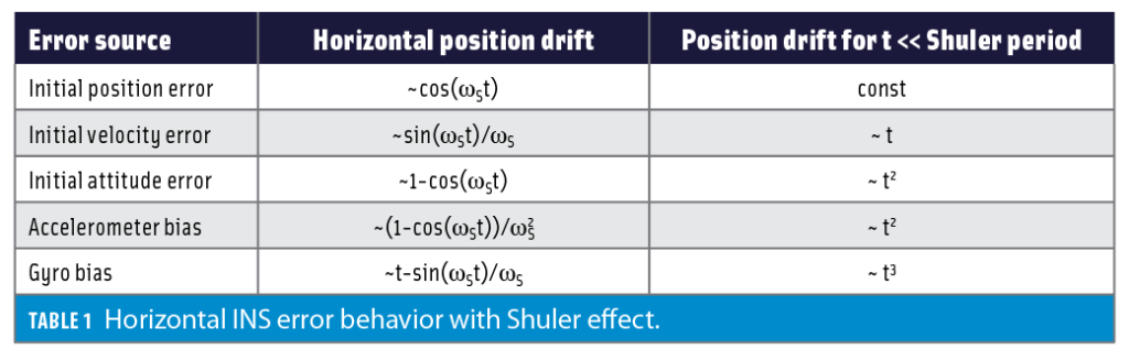
It is noted that for time intervals that are significantly shorter than the Shuler period, the error behavior is well approximated by polynomials: e.g., ~t2 and ~t3 for accelerometer and gyro bias components, respectively, as we derived previously. It is also worth mentioning that gyro bias is the only error source that leads to unlimited position error growth (even though over longer periods of time the growth becomes linear rather than cubic thanks to the Shuler feedback mechanism).
Unlike the horizontal channel, the vertical INS channel is inherently unstable. The reason is that gravitational acceleration reduces as the distance from the Earth surface increases. As a result, vertical position error is further amplified through the gravity addition rather than being dampened by it (as in the horizontal channel case). For this reason, higher-quality inertial systems that are designed to maintain stand-alone navigation over long periods of time are commonly augmented with a barometric altimeter to stabilize the vertical channel.
Sensor Noise and First-Order Gauss-Markov Models
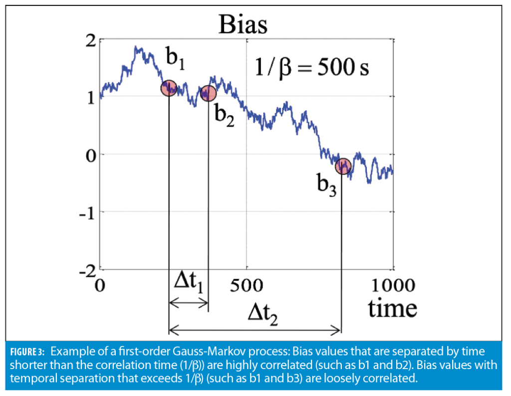
Approximation of accelerometer and gyro measurement errors by a constant bias is good for providing an insight into the key principles of INS error growth. Yet, for practical cases, it is too simplistic even for low-grade MEMS sensors. More adequate modeling of sensor measurement errors includes slow-varying bias and noise terms. Noise is represented by a zero-mean Gaussian random process. Slow-varying time bias is approximated by the first-order Gauss-Markov process. This process has an exponential autocorrelation function:

where 1/β is a time constant that is inversely proportional to the correlation time as illustrated in Figure 3.
It is noted that for gyroscopes, the noise measurement is commonly characterized by a random angular error, nδα, that is accumulated over time:

where nδw is the rate measurement noise and ∆t is the measurement update interval. Accumulated noise is often referred to as a random walk akin to accumulating steps of random (positive and negative) lengths. Assuming uncorrelated noise samples at different measurement instances, the random walk variance is:

where nδw is the rate measurement noise and ∆t is the measurement update interval. Accumulated noise is often referred to as a random walk akin to accumulating steps of random (positive and negative) lengths. Assuming uncorrelated noise samples at different measurement instances, the random walk variance is:

Other Error Sources
Other sensor-related error sources that can contribute into the inertial error budget include scale-factors, g-sensitive errors and non-linearity sensitivity errors (e.g., squared acceleration scale factors). There are also two important error sources that are not related to sensor imperfections. The first one is packaging error, more specifically misalignment of sensitive axes from a perfect mutually orthogonal sensor orientation assumed by strapdown mechanization algorithms.
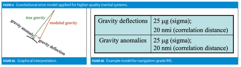
The second non-sensor error source is gravity modeling errors. For consumer-grade INS, a simple gravitational model assumes a downward pointed gravity with the absolute value of 9.8 m/s2. As the quality of inertial sensors improves, a more precise gravitational model has to be used to balance the overall error budget. In this case, the orientation and absolute value of the gravity vector are modeled as a function of position. Modeling errors are characterized by gravity anomaly and gravity deflections as illustrated in Figure 4.
Both packaging errors and gravity modeling errors can lead to substantial navigation drift even in a (hypothetical) case where perfect accelerometers and gyroscopes are used.
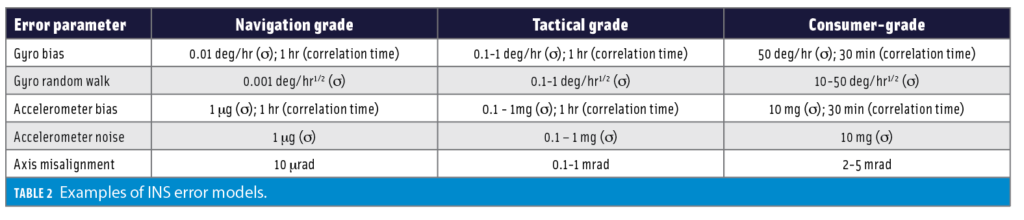
Example Error Models
Table 2 shows typical error parameters for different INS grades.
Examples of INS Error Budgets
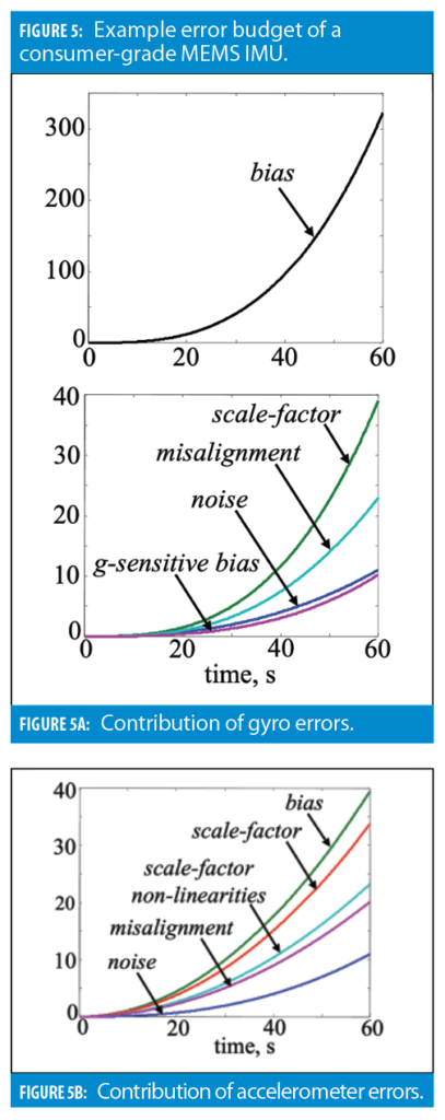
This final section provides two examples of the INS error budget. The first example is shown in Figure 5 for a consumer-grade INS. Stand-alone inertial functionality over a 1-minute interval is considered.
In this case, gyro bias is clearly the largest contributor into the position error drift, while contributions of other error sources are about an order of magnitude lower.
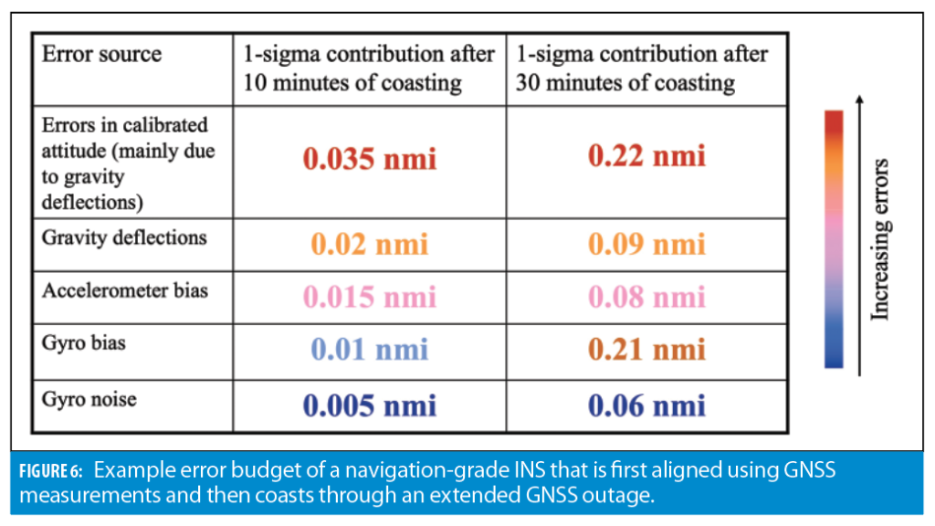
The second example is coasting with navigation-grade INS over a GNSS jamming region. In this case, a simulated flight scenario includes (a) an initial INS alignment segment where the GNSS is available (10 minutes), and (b) a complete GNSS outage (10 to 30 minutes). The inertial is first pre-calibrated using GNSS measurements (pseudoranges and carrier phase) and then switches into a stand-alone mode after GNSS becomes jammed.
Figure 6 shows the contribution of different error sources, which also includes errors in the gravitational model, with modeling parameters illustrated in Figure 4. Interestingly, in this case, gravitational errors are the major
contributor into the INS error budget after 10 minutes of coasting. Their contribution becomes more balanced with the gyro drift after 30 minutes of GNSS-denied operations. Nevertheless, in this example case, improving INS sensor performance will not significantly improve the overall system accuracy because the gravitational model has to be improved first.
Conclusion
To summarize, errors in inertial sensor measurements are accumulated over time into drift in INS navigation outputs (position, velocity and attitude). Position errors grow proportionally to (i) time3 due to gyro biases, and (ii) to time2 due to biases in accelerometer measurements. This polynomial error growth is stabilized by the Schuler effect for the horizontal channel when duration of stand-alone INS operation is comparable to 84 minutes.
Gyro bias can be generally considered as the main error contributing factor, especially for longer coasting intervals. Yet, other error sources (accelerometer bias, gyro and accelerometer noise, scale-factors and non-linearity errors) are also important for balancing the overall error budget. In addition,
sensor packaging and gravity modeling errors must be accounted for in INS error models. For example, a gravitational model error can be the main contributing factor for navigation-grade GNSS/INS when coasting over GNSS outages during relatively limited intervals of 10 to 30 minutes.