A factor-graph optimization-based GNSS positioning method uses GNSS pseudorange and Doppler observations to estimate position, velocity, and receiver clock biases. Added constraints on past and current graph nodes of the graph using time-difference observations of the GNSS carrier phase improve the accuracy, and a robust optimization method excludes multipath outliers. Experimental results reduce horizontal positioning error from 5 to 10 meters to 1.37 meters.
TARO SUZUKI
Chiba Institute of Technology, Japan
Autonomous cars and outdoor mobile robots must overcome multipath signals to achieve better than few-meters GNSS single point positioning accuracy, which is insufficient for autonomous navigation. Combining GNSS with other sensors and 3D mapping data is very complex and expensive, and there is a need for a method to improve positioning accuracy in urban environments using only GNSS.
Methods using graph-based optimization have attracted attention recently, including research in robotics and computer vision [see References]. Compared with traditional filtering approaches, the graph optimization approach generally yields better performance in multi-sensor integration.
This article focuses on a graph construction method using GNSS only, unaided by inertial navigation, to improve positioning accuracy in a multipath environment. Robustly and accurately estimating the position of a vehicle by adding a new type of constraint in the graph optimization uses a single receiver with time-relative real-time kinematic (TR-RTK) GNSS, a precise constraint between nodes of past and current nodes. In addition, adding clock biases between the multi-constellation GNSS as an estimated state and using a switchable constraint to exclude the observations of multi-GNSS pseudorange and Doppler frequency, which includes multipath errors, improves the positioning accuracy. Finally, the article evaluates this method’s accuracy using open GNSS datasets acquired in an urban environment.
Factor-Graph Optimization
Formally, a factor graph is a bipartite undirected graph that includes two types of nodes, variable nodes and factor nodes, and edges. A variable node presents the state variable Xi at i-th different moments. The edge connects the factor node and variable node and encodes the error function e(⋅), in which each edge corresponds to a single observation Zi. The optimization factor graph can be represented as:
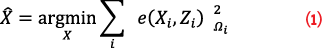
where Ωi represents the information matrix of a constraint relating to the parameters Xi and determines the weight of an error function over the entire optimization problem. We consider the GNSS positioning problem as an optimization problem by constructing a factor graph from GNSS observations.
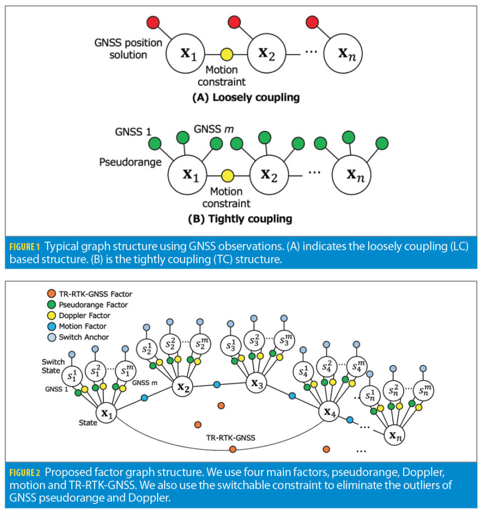
The accuracy of position estimation by factor-graph optimization depends significantly on the graph structure and the type of factors used. The graph structure shown in Figure 1 (A) is the simplest structure and directly uses the position and velocity computed by GNSS as edges. This structure is called “loosely coupling” (LC). On the other hand, the graph structure in Figure 1 (B) uses the pseudorange and Doppler observations from each GNSS satellite as edges. This structure is called “tightly coupling” (TC). As an edge between nodes, we can use the factor of dynamics such as velocity. In the case of TC, it is necessary to add the clock bias of the GNSS receiver to the estimated state. Compared to LC, TC can process the observations from each satellite independently, so outlier rejection methods such as switchable constraints can be applied to the observations of each satellite. Therefore, TC is expected to improve the positioning accuracy in multipath environments.
However, the accuracy of the pseudorange observations is at the meter level and is susceptible to multipath signals. Here we add centimeter-level TR-RTK-GNSS constraints to the TC-based graph structure using observations from a multi-GNSS constellation to achieve robust GNSS positioning in multipath environments.
We use GNSS pseudorange, Doppler, and carrier phase measurements as constraints of the factor graph. The node X estimated in epoch i is the 3D position and velocity in earth center earth fixed (ECEF) coordinates and multi-GNSS receiver clock biases and receiver clock bias rate:
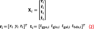
where tgps,i is the receiver clock bias of the gps satellites, and tglo,i, tgal,i, and tbds,i are the system biases including the time bias of the GLONASS, Galileo and BeiDou relative to the GPS time.
Figure 2 illustrates the structure of graph-based optimization using the proposed method. Four main factors exist: multi-GNSS pseudorange, Doppler, motion and TR-RTK-GNSS. n is the total number of estimated states, and m is the number of GNSS satellites. Unlike conventional TC, this graph structure has accurate TR-RTK-GNSS factors between distant nodes, making it possible to correct the accumulated error and estimate the accurate trajectory. We use switchable constraints to reject the multipath error of pseudorange and Doppler measurements. A set of switch variables S with components si is added to the state. The optimizer can find the best possible choice of each switch variable automatically. The switchable constraints can be thought of as an observation weight that is to be optimized concurrently with the state estimates. This proposed graph structure does not require other sensors such as an inertial measurement unit (IMU) or GNSS reference stations but is constructed using only a single GNSS receiver.
Pseudorange and Doppler Factors
Pseudorange and Doppler measurements of each satellite are used as constraints to estimate the position and velocity. We compensate the ionosphere and troposphere error in pseudorange using the Klobuchar model and Saastamoinen model as with the standard single point positioning. The satellite clock error is compensated using the broadcast ephemeris. In the case of the receiver clock error and different system biases, we included these biases in the nodes and estimated them.
For further detailed equations relating to the pseudorange, Doppler observations, ionospheric delay and motion factor (the relative constraint between time-series nodes), see the ION GNSS+ 2021 paper on which this article is based, at ion.org/publications/browse.cfm.
TR-RTK-GNSS Factor
This study attempts to construct loop-closure edges using the TR-RTK-GNSS technique. Previous GNSS pseudorange and carrier-phase measurements are stored and used to construct double-difference measurements between the past and current measurements. The baseline vectors pointing from the past epoch to the current position are determined exactly. We use these baseline vectors as the loop-closure edges in the graph. The GNSS carrier phase measurement of satellite k in epoch i is denoted as Φik. Φik is given by:

where rik is the range from the receiver to the satellite k, λ is the signal wavelength, Nik is the integer ambiguity, c is the speed of light, δti and δTik are the receiver and satellite clock biases, respectively, Iik and Tik are the ionosphere and troposphere errors, and εik is the carrier phase measurement noise. In general, when two receivers are used, mutual error terms exist in the measurements from the same satellite. The ionosphere, troposphere and satellite clock bias errors may be eliminated by differencing the base and rover receiver measurements. In contrast, we consider the time-differential carrier phase using a stand-alone GNSS receiver. (Further discussion will be found in the ION GNSS+ paper cited earlier.)
The GNSS carrier phase measurements are biased by an unknown integer ambiguity. This ambiguity will be a time-invariant constant, provided that there is a continuous phase lock to the respective GNSS satellite in the receiver phase lock loop. However, the GNSS carrier phase measurements are sensitive to signal shadowing. In urban environments, tall buildings and overpasses are likely to cause complete signal obstruction. In these situations, cycle slip of the GNSS carrier phase occurs, and the integer ambiguity will not be a time-invariant constant. For this reason, we do not eliminate integer ambiguity in the time difference computation.
The form of the observed equation of TR-RTK-GNSS is similar to that of normal RTK-GNSS. Therefore, the baseline vectors and ambiguity are estimated using the ambiguity estimation method used in RTK-GNSS. In general, the ambiguities are first fixed to float numbers using a Kalman filter or a least-squares method from the double-difference carrier phase measurements in single or multiple epoch. Then float ambiguities are corrected with the integer ambiguities, and the accurate baseline vector can be computed using the estimated integer ambiguities. We use the LAMBDA method to estimate the integer ambiguities, and the precise relative position between the past and current epochs can be estimated.
We create a combination of epochs within the past few minutes from the current epoch and execute the proposed method. If TR-RTK-GNSS can correctly estimate the carrier phase ambiguity as an integer, we add all the TR-RTK-GNSS constraints to the graph. We do not add the constraint if the integer carrier phase ambiguity cannot be solved by the LAMBDA method.
Optimization
We add all the constraints into the pose graph. We use the switchable constraints, and the switch value of each satellite is estimated simultaneously. This is shown in Figure 2. The switch variable takes a value between 0 and 1 and serves as a weight for the GNSS observations. When the pseudorange residuals become large, the switch’s value becomes small, and it is possible to automatically exclude the pseudorange and Doppler observations that contain multipath errors.
The objective of localization is to find the optimal state variables that guarantee the minimized aforementioned error function. We use the Dogleg optimizer to obtain the optimal solution of the aforementioned error function. Finally, we can estimate the accurate vehicle’s trajectory. The proposed method using TR-RTK-GNSS facilitates improving positioning accuracy in applications without using any additional sensors and data from a GNSS base station.
Experimental Setup
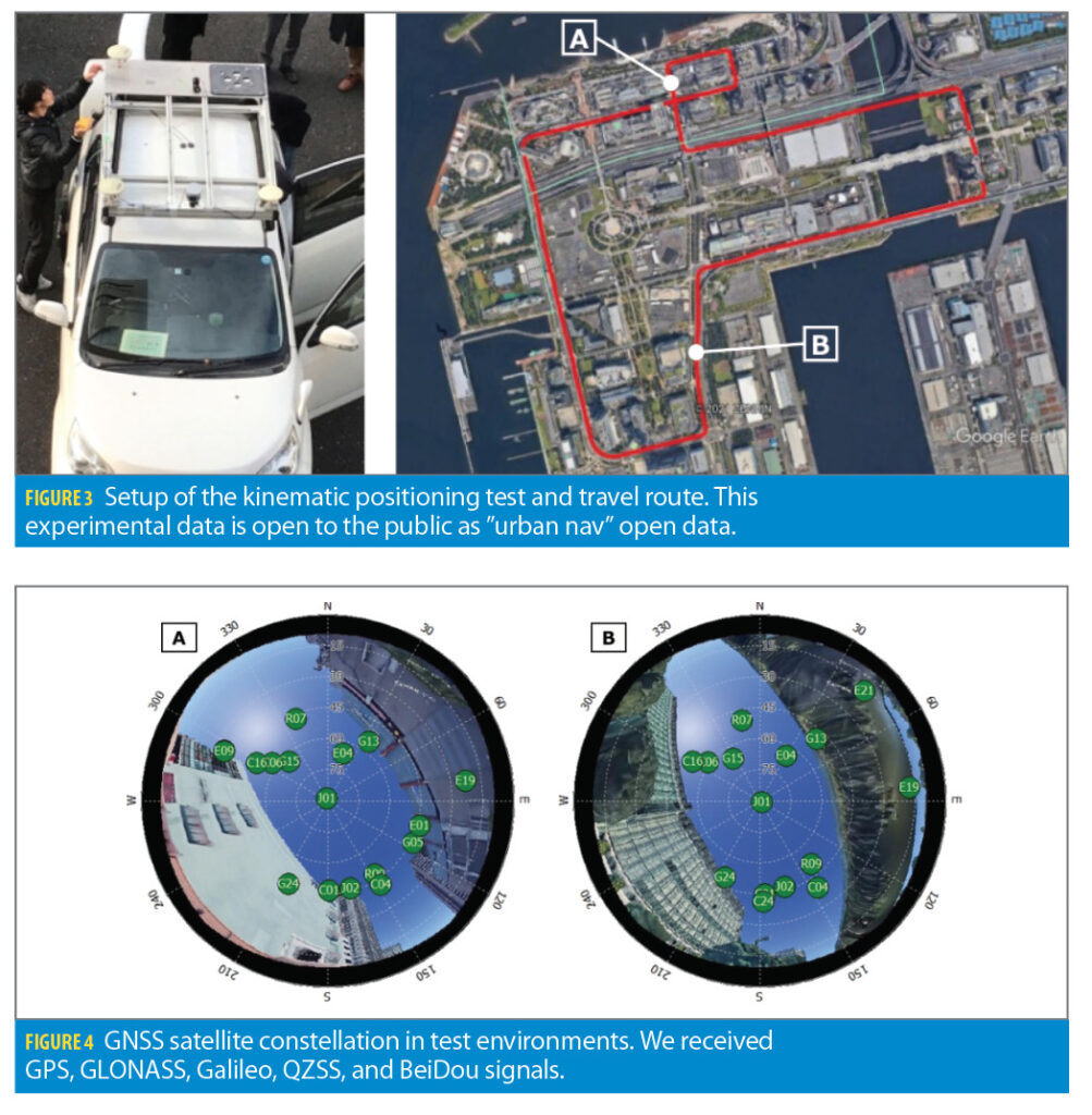
To confirm the effectiveness of the proposed method, we conducted kinematic positioning tests using a vehicle in actual urban environments. Figure 3 shows the setup of the positioning test and the travel route. Buildings standaround the travel route, and therefore the environment is susceptible to satellite masking.
For the evaluation, a position estimation system for land vehicles that uses a multiple-frequency GNSS receiver and high-grade IMU, was used to estimate the reference positions as a ground truth. The accuracy of the absolute position estimation is centimeter accuracy according to the catalog specification. Therefore, it is accurate enough to be used to obtain the ground truth to compare the proposed methods. This experimental data is open to the public as “UrbanNav” open data [16], and can be used by anyone.
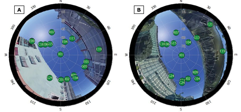
Figure 4 shows the actual locations of the GNSS satellites observed at locations “A” and “B” on the travel path shown in Figure 3. Here, G, R, J, E, and C indicate GPS, GLONASS, QZSS, Galileo, and BeiDou, respectively. Using ground truth location information, we extracted 3D information of the surrounding area from Google Earth, converted it into a virtual fisheye image, and projected the received satellite position. As shown in Figure 4 (B), part of the course is shielded by an elevated railroad. As can be seen in Figure 4 (A), multipath signals are received from satellites hidden behind buildings. These multipath signals have a significant impact on positioning accuracy.
Evaluation and Results
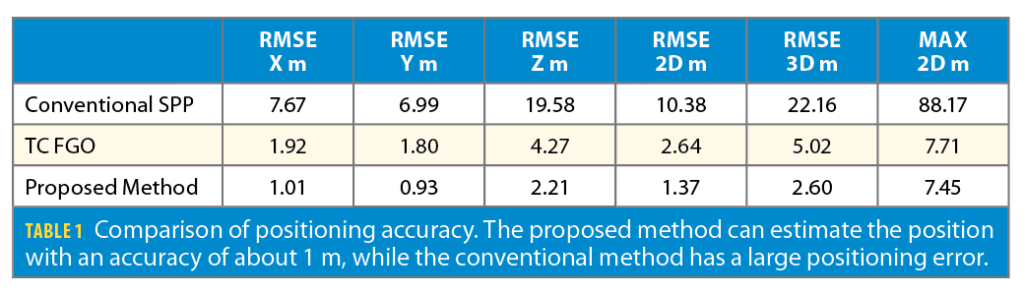
We compare the proposed graph optimization-based positioning error with the conventional single point positioning (SPP) result using the Kalman filter. We also compare the positioning error of general TC-based graph optimization. TC-based graph optimization uses multi-GNSS observations, and the TR-RTK-GNSS factor is removed from the proposed method. By comparing these positioning results, we evaluate the effectiveness of the proposed method.
We used the GTSAM for graph optimization backend, and RTKLIB for GNSS general computation. The proposed method is implemented using MATLAB, and the performance evaluation was conducted in post processing.
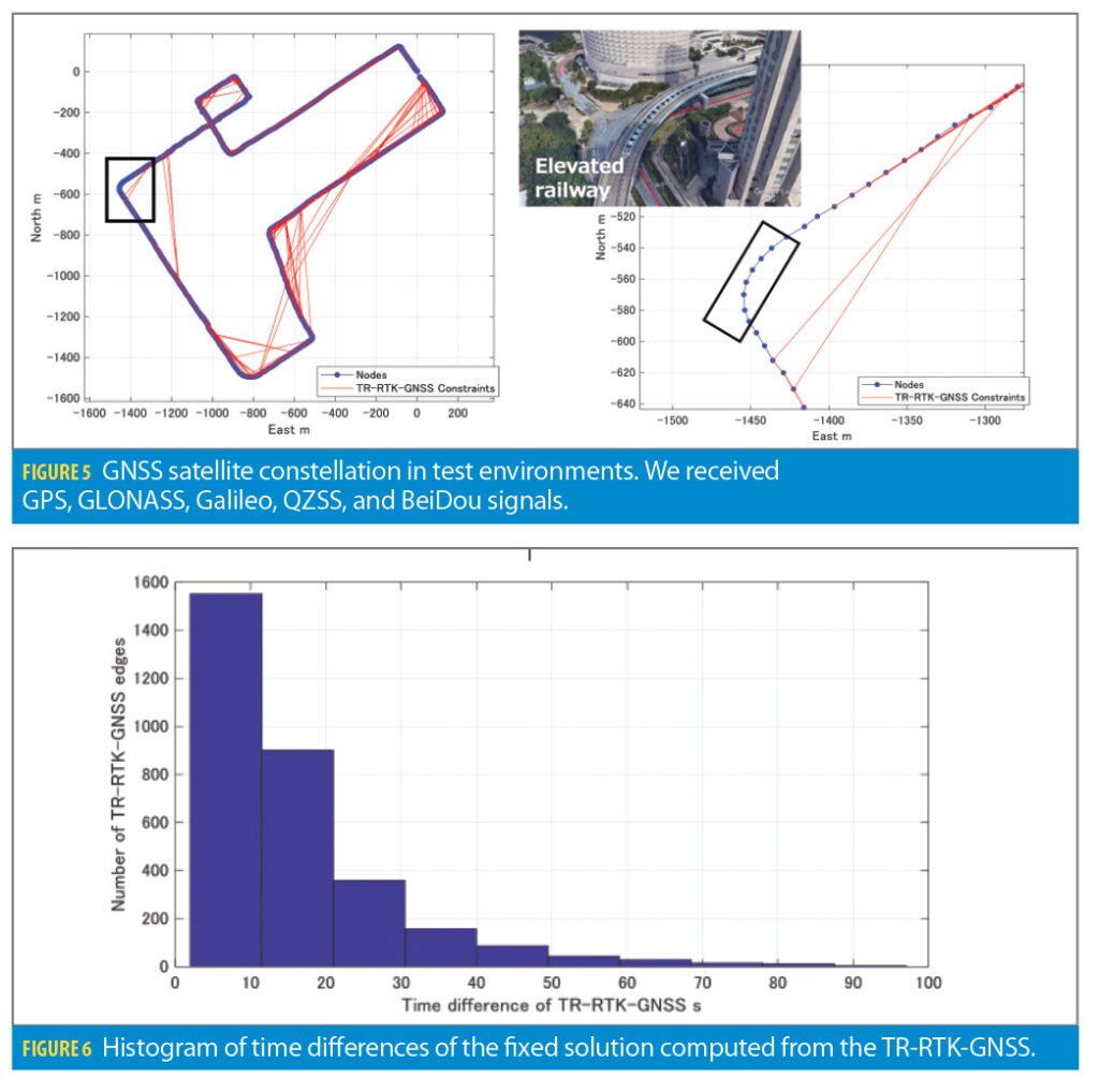
Figure 5 shows a visualization of the TR-RTK-GNSS factor in the graph structure constructed by the proposed method. The blue circles in the figure represent the nodes of the graph, and the red lines represent the edges with TR-RTK-GNSS Factor. The figure shows an enlarged view of a part of the course, where we can see that the constraints are added between distant nodes. Because the TR-RTK-GNSS constraints are added only when the carrier phase ambiguity is estimated to be solved correctly, some sparse constraints are added between the nodes. In environments where GNSS satellites are shielded, such as under an elevated railroad, no TR-RTK-GNSS constraint is generated. The black square area in the figure is the case where the vehicle passed under the elevated railroad. By solving the ambiguity of the carrier phase observation, the exact constraints between the nodes can be added before and after the passage of the elevated railroad by the TR-RTK-GNSS technique.
Figure 6 shows the histogram of the time differences of the fixed solution computed from the TR-RTK-GNSS technique. The maximum time difference was 95 s in this test, which was the limitation for the construction of the loop-closing constraint by the proposed TR-RTK-GNSS technique. However, the ability to create edges between distant nodes by solving for carrier phase ambiguity, as shown in Figure 5, will contribute to the higher accuracy of GNSS positioning in urban environments.
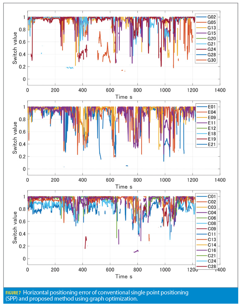
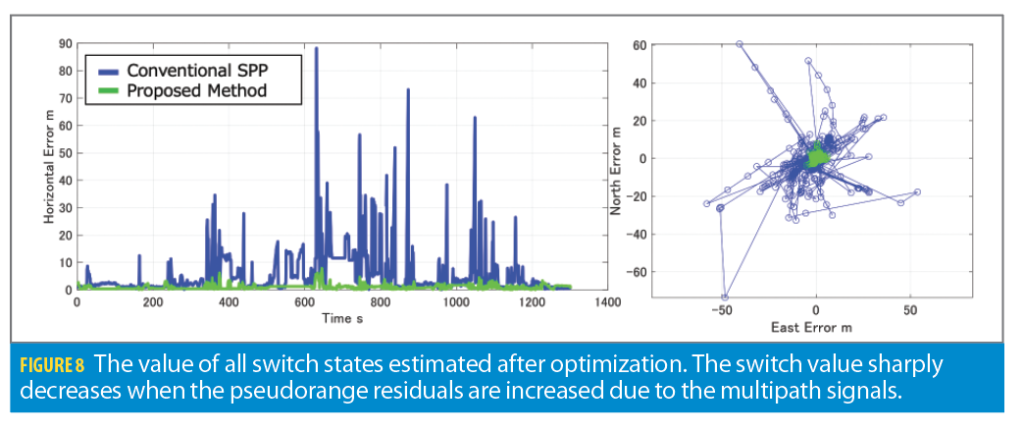
Figure 7 shows the horizontal positioning errors of each method. The blue line indicates the positioning error of SPP, and the green line indicates the proposed method. We can see the SPP has large errors in several ten meters because of the multipath. However, the proposed method can reduce the positioning errors. This result shows the multipath rejection scheme and TR-RTK-GNSS constraints of the proposed graph optimization allow us to estimate highly accurate positioning in urban environments.
Table 1 shows the positioning error of each method. Compared with the conventional SPP, the maximum positioning error is reduced from 88.2 m to 7.45 m by the proposed method. The horizontal root mean square error (RMSE) is also reduced from 10.38 m to 1.37 m. Compared to the TC-based graph optimization, the contribution of the TR-RTK-GNSS factor further improves the positioning accuracy.
Figure 8 shows the value of the estimated switch state of the GPS satellites after the optimization. Each line in the figure indicates the switch state of each satellite. This switch value indicates the GNSS measurement qualities. It is apparent that switch variables sometimes drop and close to zero. This supports the understanding that the optimization could clearly recognize the outlier measurements and distinguish them from the inliers. The only inlier pseudorange and Doppler measurements are used to estimate the vehicle positioning and velocity; as a result, the proposed method can estimate the accurate position in multipath environments.
Conclusion
A high-accuracy positioning method in urban environments with multipath uses a graph optimization method employing only GNSS. The method rejects outliers in multi-GNSS pseudorange and Doppler observations by using switchable constraints and constructs a graph that fully utilizes multi-GNSS by including the clock bias between multi-GNSS in the state. Furthermore, we added a constraint between distant nodes by TR-RTK-GNSS using the time difference of GNSS carrier phase observations to improve the GNSS positioning accuracy. The accuracy of the proposed method was evaluated using GNSS data sets in an urban environment, and the results show the proposed method has the highest accuracy compared to the general single point positioning, loose-coupled combined and TC combined methods.
In future research, we will work on how to optimize the proposed graph structure in real-time using incremental smoothing and mapping (iSAM) and other methods. This will allow us to use the proposed method for real-time position estimation, such as navigation for automated driving. In addition, by combining the proposed method with inertial navigation systems, we aim to improve the accuracy in environments where GNSS cannot be used, such as tunnels and under elevated tracks.
Manufacturers
The POSLV from Applanix was used to estimate ground truth in the experiment.
References:
(1) N. Sunderhauf and P. Protzel, “Switchable constraints for robust pose graph SLAM,” in IEEE international conference on intelligent robots and systems, 2012, pp. 1879–1884.
(2) D. Chen and G. X. Gao, “Probabilistic graphical fusion of LiDAR, GPS, and 3D building maps for urban UAV navigation,” Navigation, Journal of the Institute of Navigation, vol. 66, no. 1, pp. 151–168, Jan. 2019.
(3) N. Sünderhauf, M. Obst, G. Wanielik, and P. Protzel, “Multipath mitigation in GNSS-based localization using robust optimization,” in IEEE intelligent vehicles symposium, 2012, pp. 784–789.
(4) W. Li, X. Cui, and M. Lu, “A robust graph optimization realization of tightly coupled GNSS/INS integrated navigation system for urban vehicles,” Tsinghua Science and Technology, vol. 23, no. 6, pp. 724–732, Dec. 2018.
(5) R. M. Watson and J. N. Gross, “Robust navigation in gnss degraded environment using graph optimization,” in 30th international technical meeting of the satellite division of the institute of navigation, ION GNSS 2017, 2017, vol. 5, pp. 2906–2918.
(6) W. Wen, T. Pfeifer, X. Bai, and L.-T. Hsu, “Factor graph optimization for GNSS/INS integration: A comparison with the extended kalman filter,” NAVIGATION, vol. 68, no. 2, pp. 315–331, 2021.
(7) T. Suzuki, “Time-relative RTK-GNSS: GNSS loop closure in pose graph optimization,” IEEE Robotics and Automation Letters, vol. 5, no. 3, pp. 4735–4742, 2020.
(8) F. R. Kschischang, B. J. Frey, and H. A. Loeliger, “Factor graphs and the sum-product algorithm,” IEEE Transactions on Information Theory, vol. 47, no. 2, pp. 498–519, 2001.
Author
Taro Suzuki is a chief researcher at Chiba Institute of Technology, Japan. He received his Ph.D. in engineering from Waseda University, worked as a postdoctoral researcher at Tokyo University of Marine Science and Technology and as an assistant professor at Waseda University. His current research interests include GNSS precise positioning in urban environments. Another ION GNSS+ 2021 paper of his, ” Global Optimization of Position and Velocity by Factor Graph Optimization,” won first place in the Google Smartphone Decimeter Challenge.


