Authors: Frank van Diggelen and Mohammed Khider
Google has publicly released GNSS Analysis Tools to process and analyze GNSS raw measurements from your phone. These tools enable manufacturers to see in detail how well the GNSS receivers are working in each particular phone design and thus improve the GNSS design and performance in their phones. Also, with the tools publicly available there is significant value for app-developers, researchers and educators. Here, the authors show what these tools do, and how they reveal details of receiver and signal behavior that are not possible to observe without raw measurements.
In Android Release N (“Nougat”), Google introduced APIs giving access to GNSS raw measurements from your phone. Now Google has publicly released Analysis Tools to process and analyze these measurements.
Android now powers more than two billion devices, and Android phones are made by many different manufacturers. The analysis tools enable manufacturers to see details of how the GNSS receivers are performing in different phone designs. Also, with the tools publicly available app developers, researchers, and educators can use them to develop, build and teach.
This article shows what these tools do, and how they reveal details of receiver and signal behavior that are not possible to observe without raw measurements.
We begin with the basic operation of the tools, then describe the raw measurements, derived data, interactive controls, and custom parameters. Additionally, we’ll work through three examples, showing how you can use the tools for easy, but fairly sophisticated, analysis. Next, we’ll cover report generation, and on-phone analysis. Then we’ll describe some specifics of dual frequency analysis, including the mission planner. Finally, we’ll describe where to download the tools, open source code on Github, frequently asked questions and how to provide feedback.
Basic Operation
The basic operation of the tools is: users log raw GNSS Measurements with their phones, and analyze on their desktops.
The desktop tools run on Windows, Linux and Mac OS.
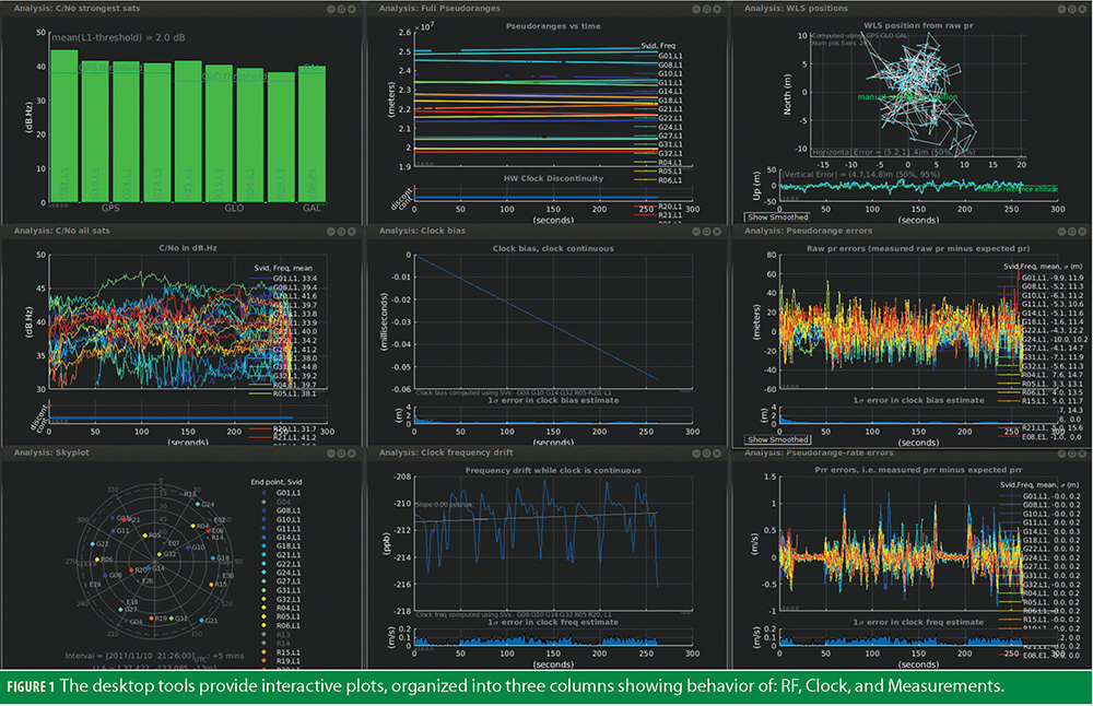
The RF column (Figure 1) shows:
a) The strongest four satellites from each constellation
b) The time plot of C/N0 of all satellites
c) The skyplot of satellite positions
The Clocks column shows:
a) The pseudoranges
b) The offset frequency of the receiver clock. This is computed using a reference position — either:
i) Automatically computed mean position
ii) User entered lat,lon,alt
iii) NMEA file with truth reference PVT
This is the first major benefit of raw measurements:
you can see the receiver clock behavior to better than 1ppb (part per billion) precision. This is a really important thing to see when you are making a phone — because any heat source near the reference oscillator inside the phone may cause the clock error to ramp rapidly. And the best way to see this, in the actual phone, is to use the raw measurements like this.
c) The offset of the standby clock that keeps time if the receiver duty cycles the primary oscillator
The Measurements column shows:
a) The weighted least squares (WLS) position results obtained from the raw and smoothed pseudoranges
b) The residual errors of each pseudorange, raw and smoothed
c) The residual errors of each pseudorange-rate (-Doppler) measurement
This is the second major benefit of raw measurements: you can see the errors of each measurement, and this allows significant insight into the signal environment and receiver behavior.
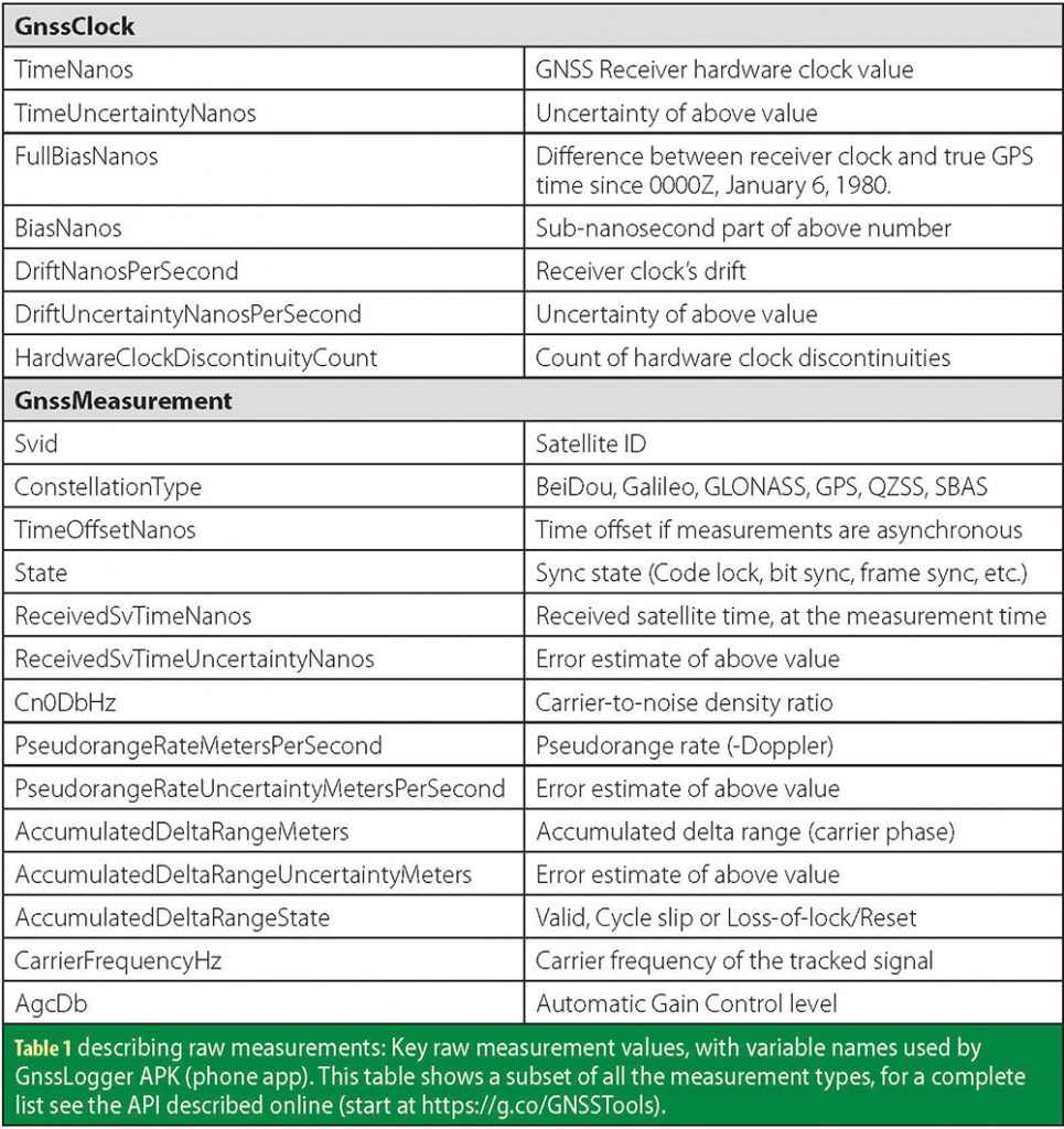
Raw Measurements and Derived Data
The Android API describes truly raw measurements. One of the first things you might notice when you examine the API (see Table 1) is that there are no pseudorange measurements. This is because pseudorange is not a raw measurement, it is derived from received satellite time (ReceivedSvTimeNanos). This is something of a paradigm shift for readers brought up on survey receivers that output pseudoranges. But remember that the primary purpose of the GNSS Raw Measurements API is to observe (and thus improve) the operation of the GNSS receiver, and that is why the APIs describe the fundamental raw values. It is our hope and intent that developers will create apps that build on these measurements, providing many derivations of the raw measurements. Indeed this has already started with apps to do PPP and generate RINEX data from your phone (see Additional Resources at the end of this article).
How do you get pseudoranges from these values? The analysis tools will do it for you, and if you want to do it yourself, see the open-source code. But as a summary:
pseudorange = (tRx- tTx)*c,
tTx = ReceivedSvTimeNanos [ns],
tRx = (TimeNanos +
TimeOffsetNanos) –
(FullBiasNanos+BiasNanos)
– weekNumberNs [ns],
where
weekNumberNs =604800e9
*floor(-FullBiasNanos/604800e9)
This summary is correct for GPS when time of week is known (State = STATE_TOW_DECODED or STATE_TOW_KNOWN). For other constellations and/or other states you must take care of details such as modulo milliseconds, and system time offsets. This is beyond the scope of this article, but these details are handled by the analysis tools and the resulting pseudoranges are available in the derived data.
The Desktop Analysis Tools compute smoothed pseudoranges as follows.
For intervals where the hardware clock is continuous, the smoothed pseudorange for a particular satellite signal is the least squares solution x to the matrix equation:
Wy = WAx
where
y = [column vector of raw pseudoranges
column vector of prr],
prr is the measured pseudorange-rate or, if available, the
change in carrier phase divided by Δt,
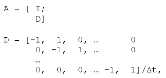
Δt is the time interval between measurements
W is a diagonal matrix, with Wii = 1/σ(yi)
That is, the smoothed pseudorange is the minimum variance linear estimator of the true pseudorange, given the measurements and variances of pseudorange (pr) and pseudorange-rate (prr), and zero-mean uncorrelated errors. In plain English, this is the best estimate we can get by post-processing all the available information.
Derived Data
Once you have processed a log file with the desktop tools, you can save all the derived data to a comma-separated text file. The derived data file includes: satellite azimuth and elevation, raw pseudorange, smoothed pseudorange, and the residual errors of the raw and smoothed pseudoranges (residual errors derived from the known reference positions). The derived data also contains the receiver clock bias and frequency error. From this file you can regenerate all the line plots and the skyplot produced by the Desktop Analysis Tools.
The tools provide interactive controls, and custom parameters. We’ll introduce these now and then show three examples of how to use them for analysis.
For greater control you can set custom parameters by including a text file: CustomParam.txt in the same directory as your log file. In this file you can declare the satellite(s) to be used for computing the clock errors (Figure 2).
Following are three examples that illustrate how to use the interactive controls.
![]()
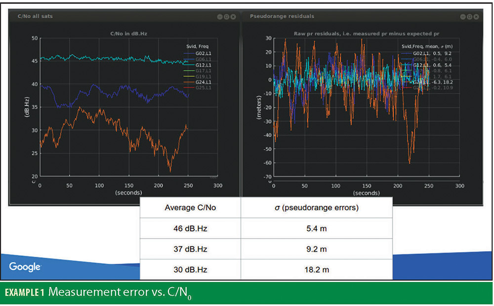
Example 1: Measurement error vs C/NO.
The tool lets you select any subset of the visible satellites. In this case we’ve chosen three with different C/N0: Strong, Medium, Weak (Example 1). You can read the computed raw pseudorange errors directly from the plot, including mean and standard deviation. You can clearly see two things:
1) the relationship of C/N0 to pseudorange errors
2) the increased filtering that the receiver does to track the weaker signals, combined with the fading caused by multipath, especially on weak signals — note the increasing time constants of the errors.
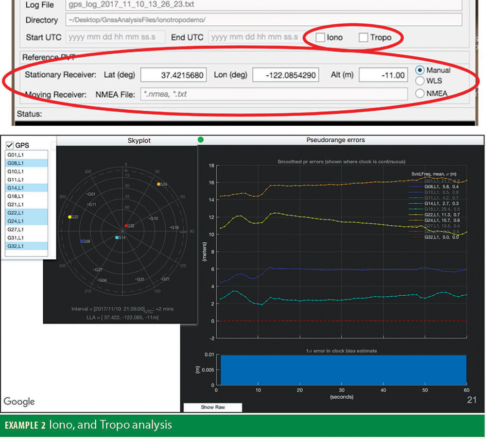
Example 2: Iono, and Tropo analysis
In this example we process data collected at a known point, under open sky, away from any buildings or reflecting surfaces. We disable Iono and Tropo models by unchecking the respective boxes on the control panel, and we set the Reference PVT to the known true position of the receiver (Example 2).
The pseudorange error plots will now include the sum of Ionosphere, Troposphere, and Orbit errors. For GPS and Galileo, the typical orbit error in the broadcast ephemeris are now less than 0.5 meters (see Additional References), so the rest of the pseudorange error will be dominated by Iono+Tropo delay.
There is one thing left to do: specify which satellite to use for computing the clock error. Ordinarily the analysis program will automatically select several satellites for this. But, in order to observe relative error of iono and tropo we select a single reference satellite for computing the receiver clock. The pseudorange error on this satellite will be zero, by definition, and the errors on the remaining satellites will be the difference between their errors and the reference satellite. We choose the highest satellite, and specify it in a text file CustomParam.txt:
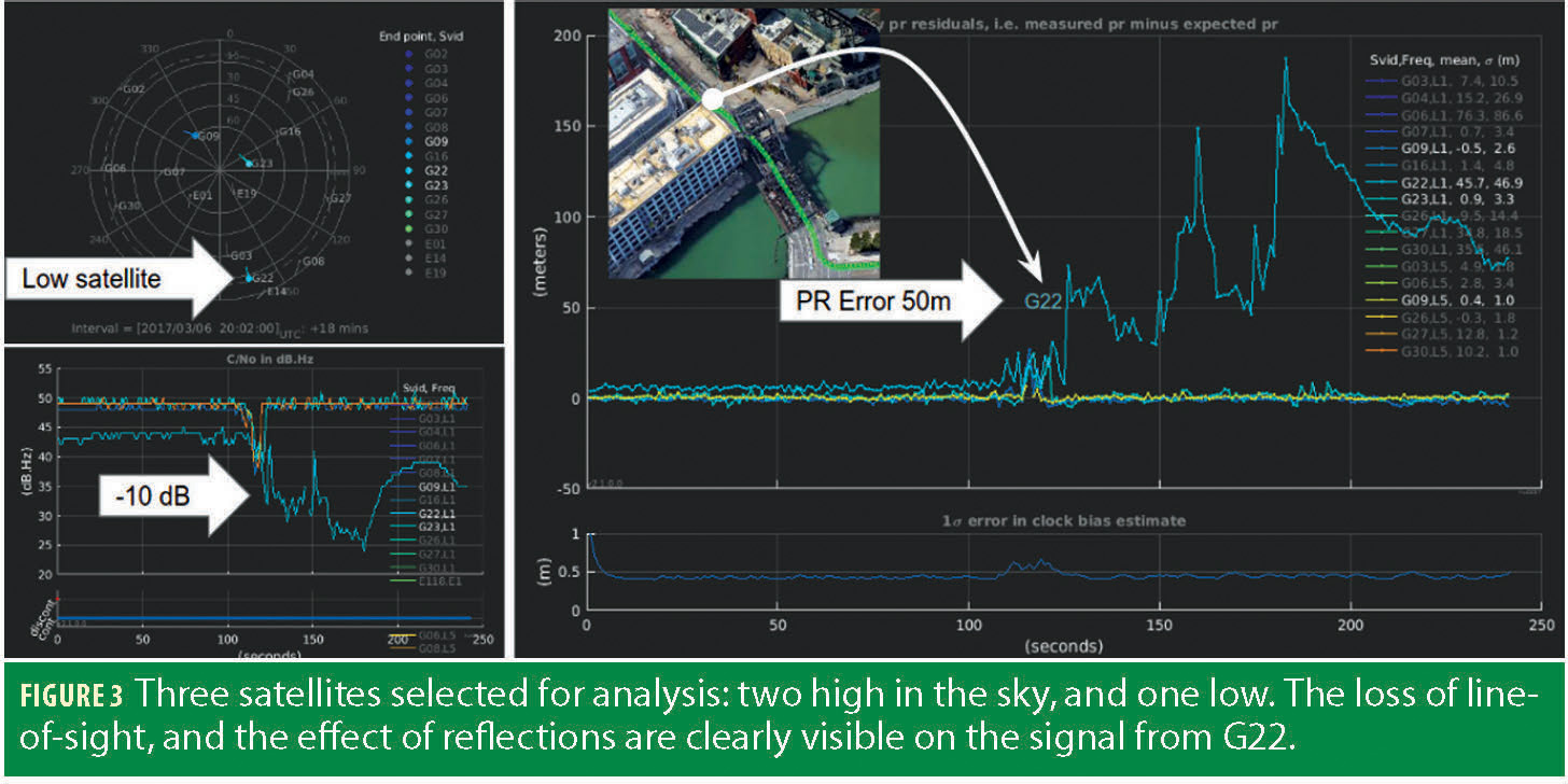
You analyze measurement errors from a moving receiver by supplying an NMEA truth reference file. The Analysis Tool reads the NMEA file and extracts the GGA messages (for 3D position) and RMC messages (for velocity). With this information the Tool can compute clock offsets and frequency, and measurement errors for pseudoranges and pseudorange-rate.
As the car drives into the city from bottom-right towards top-left, we see a sudden and dramatic change in C/N0 for the low satellite, and at the same time, a large increase in pseudorange error (Figure 3). While the error on the other satellites remains small.
So, the question is: what happened to this satellite GPS PRN 22?
Multipath — yes, but not classic multipath (with line-of-sight and non-line-of-sight signals overlapping), rather, what we see here are pure reflections. How do we know that? Because we can see from the skyplot, and the Google Earth image that this satellite is completely blocked by the building to the south of the car; combined with the C/N0 and PR error plots we can see that the signal that is tracked is something reflected from across the street.
As these examples show, in just a few minutes you can do fairly sophisticated analysis at a level that, until now, was inaccessible to anyone but the chip manufacturers themselves.
Having done this we run the analysis, and, in this example, pick five satellites with increasing elevations:
For these five satellites we observe the expected trend of greater atmospheric delay with decreasing elevations. The difference between the delay for the highest satellite (PRN 32, at 80°) and the lowest (PRN 24, at 7°) is approximately sixteen meters. In general there will be other errors (such as noise, and multipath) and at times they may be larger than the atmospheric delays. So not all signals will be this well behaved, but you can quite easily see the expected trend in most datasets.
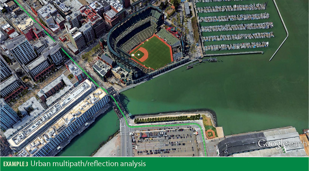
Example 3: Urban Multipath/Reflection analysis
You can observe the individual effect of multipath and/or signal reflections on each measurement. As an example, here is a drive test in San Francisco — you can see the San Francisco Giants baseball stadium in the image.
The green dots here show the truth reference obtained from a GNSS inertial navigation system. We will analyze the GNSS measurements from a smartphone chip.
On-Phone Analysis
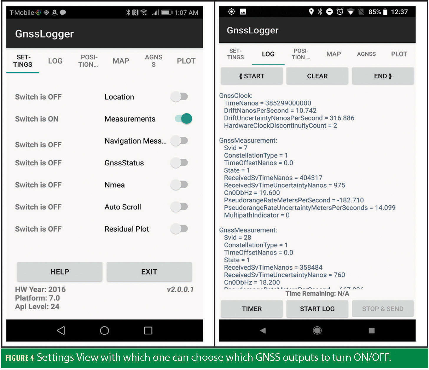
You can also do some basic analysis directly on the phone, using the Gnss-Logger App. This app was developed to:
- Exercise and validate the applicationfacing Android GNSS APIs
- Compute real-time (least-squares) position from raw measurements
- Collect data for offline analysis
The Settings View also shows important device related info such as the GNSS HW Year, Android Platform Number, Android Api Level and GnssLogger version. Log View in which the switched ON GNSS outputs will be shown (Figure 4). This view also adds the capability to log the GNSS data for offline processing and as well to send the logged files via email or other sharing options.
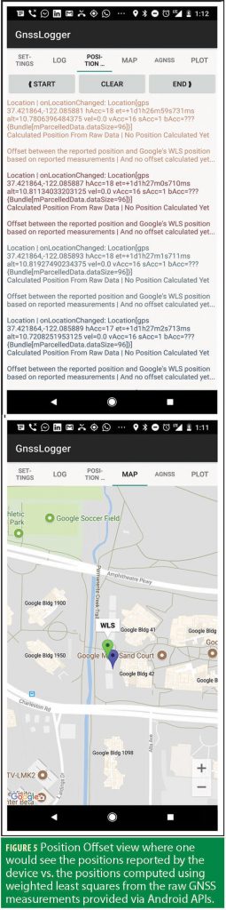
The offset between the two positions is also shown (Figure 5). As the device location is generally filtered, offsets of 5-10 meters may occur between device location and WLS (weighted least squares) location; even in open sky. With even higher offsets expected as the device moves to urban areas, or indoors.
Map view where one would see on Google Map the position reported by the device vs the weighted least square position (Figure 5, bottom).
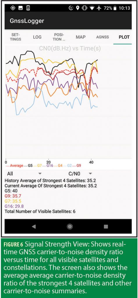
The Signal Strength View is shown in Figure 6. The Residual Error plot is shown in Figure 7, using ground truth location entered by the user. If the ground truth-location is unknown, the average reported device location can be used as ground-truth. The window over which the ground-truth-location is averaged varies based on the user activity (e.g. standing, walking, running and driving).
Multi-Frequency, Multi-Constellation
The tools support multi-constellation (GPS, GLONASS, Galileo, BeiDou and QZSS) and multi-frequency. Specifically, with the advent of L1L5 receivers for smartphones, v2.6.0.0 of the tools includes features specific to analyzing the quality of L5/E5 measurements.
If L1/E1 and L5/E5 measurements are present, then the bar chart of C/N0 shows both L1/E1 and L5/E5 signals, as well as the mean difference between L1 and L5. One of the challenges of implementing L5 in a phone is the L5 antenna, and the tools show the presence and magnitude of any RF losses. Also, the pseudorange error plots show the group delay between signals on different frequencies.
The skyplot and control panel also show which satellites signals have been tracked (e.g. L1,L5, or E1,E5a, etc).
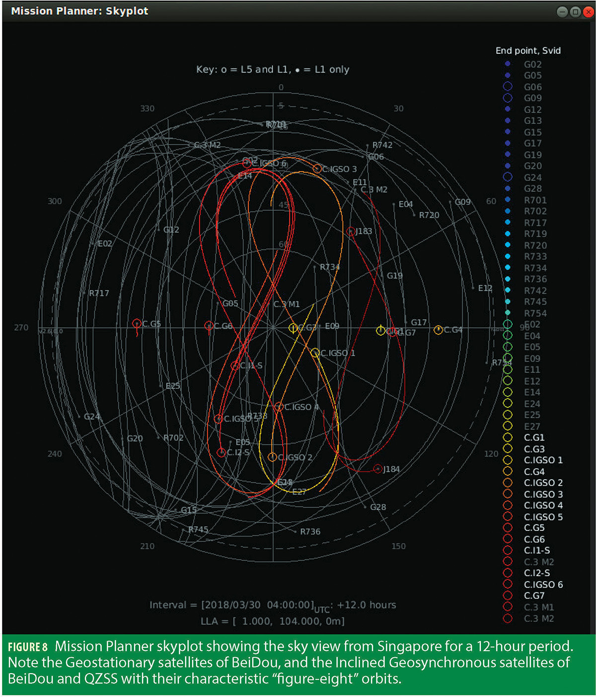
Mission Planner
The tools include a Mission Planning feature, showing which satellites will be visible from any location at any time. In particular, the Mission Planner highlights satellites with L5/E5 signals, so you can plan multi-frequency testing at appropriate times.
For example, Figure 8 shows the Mission Planner skyplot as viewed from Singapore for a 12-hour period. The GEO and IGSO satellites of BeiDou and QZSS have been selected from the control panel.
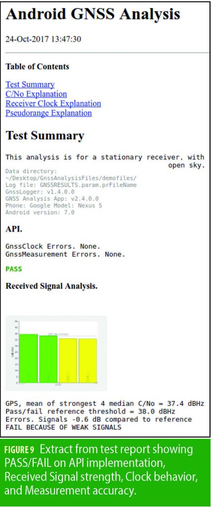
Receiver Test Report
The tools provide automatic test reports of receivers. Click “Make Report” to automatically create the test report. The report evaluates the API implementation, Received Signal, Clock behavior, and Measurement accuracy. In each case it will report PASS or FAIL based on the performance against known good benchmarks. This test report (Figure 9) is primarily meant for the phone manufacturers to use as they iterate on the design and implementation of a new phone.
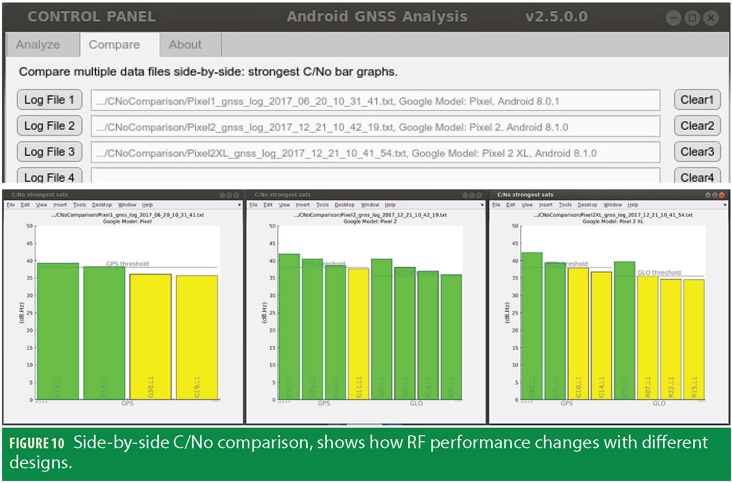
Compare Log Files
You can load multiple files and do sideby-side comparison of C/N0. The “Compare” tab lets you load several different log files to compare against each other.
The [Plot C/N0] button then produces side-by-side plots of the strongest satellites from each log file (Figure 10).
To Download the Tools and Open-Sourced Code
The compiled tools run on Windows, Mac and Linux. They have been publicly released by Google, and are available free for download at: https://g.co/GNSSTools
Open-sourced Java code is available for the GnssLogger app, and open-sourced Matlab code is available for the GPS-only part of the desktop analysis. The point of this open-source code is to help developers create their own apps, and also to provide a template for how certain values are computed (such as pseudoranges, discussed above). We will evolve the analysis tools in response to user requests, but we do not intend to open source all the code for the desktop tools beyond what is already available.
Manufacturers
In Example 3, the green dots showing the truth reference are obtained from a NovAtel SPAN system from NovAtel Inc., Calgary, Alberta, Canada. The dual frequency measurements are obtained from the BCM47755 chip from Broadcom Corp., Irvine, CA. The GnssTools smartphone app, and GNSS Analysis desktop tools are from Google Inc., Mountainview, CA.
![]()