 Figures 1 – 10
Q: Do modern multi-frequency civil receivers eliminate the ionospheric effect?
Q: Do modern multi-frequency civil receivers eliminate the ionospheric effect?
A: It is common knowledge in the GNSS community that the ionosphere is dispersive in the L-band, meaning the refractive effects on the carrier phases are proportional to the wavelengths of the carriers, in turn causing differential variation in the measured codes and phases of the various navigation signals transmitted by the satellites. Use of multiple signals of distinct center frequency transmitted from the same GNSS satellite allows direct observation and removal of the great majority of the ionospheric delay, and gives the impression to users that the ionosphere may not be a problem for modernized receivers. While the general assumption of nearly perfect correlation between the effects measured on multiple independent signals is correct in normal conditions, it does not appear to hold in the presence of ionospheric scintillation.
High and Low Latitude Scintillation Effects
Scintillation refers to random fluctuations in the received wave field strength (“signal fading”), as well as phase and group delay caused by the irregular structure of the propagation medium. Ionospheric scintillations are random rapid variations in the intensity and phase of the received signals resulting from plasma density irregularities in the ionosphere.
Many of the important contributors to ionospheric scintillation are already known, such as the variation of scintillation activity with magnetic activity, geographic location, local time, season, and the 11-year solar cycle.
The most significant and frequent scintillation activity including both phase and amplitude variations is observed in low latitude regions within about 15° of the Earth’s magnetic equator, particularly in the hours after local sunset. In high latitude regions scintillation is frequent but generally less severe in terms of signal tracking disruptions than that in the equatorial regions. The high-latitude environment can be divided into two subregions, the polar caps (regions around the magnetic poles) and the auroral zones (approximately circular regions around the two geomagnetic poles located at about 67° north and south geographic latitudes, and about 3° to 6° wide). Of these, the polar cap experiences both amplitude as well as phase scintillation activity, while mainly phase scintillation is observed at high latitude auroral regions.
In mid-latitude regions scintillation is rarely observed, but during intense ionospheric storm conditions phenomena can extend into the mid-latitudes.
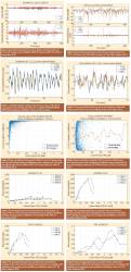
Figures 1 and 2 (see inset photo, above right, for all figures) show examples of ionospheric scintillation as observed on the detrended signal intensity (effectively power) and detrended carrier phase measurements at 69.5° latitude (Tromsø, Norway) and 21° latitude (Hanoi, Vietnam), respectively. In the particular event shown in Figure 2 the depth of fades reaches 43 decibels (dB) on L1CA which is severe by any metric, and is a substantial qualitative difference from the high-latitude phase scintillation events where only very weak fading activity is typically observed. It should be noted that ionospheric activity is more dependent on the geomagnetic latitude of the user than the geographic latitude. While it might be clear that Tromsø station is located in the auroral region, the Hanoi station has somewhat lower geomagnetic latitude than geographic latitude and is in fact located within the equatorial zone.
Since ionospheric scintillation is essentially a rapid variation in the apparent ionosphere it is easy to assume that the typical approaches applied for removing ionospheric influence will be effective during scintillation.
Ionosphere-Free Combination
The advantage of multi-frequency GNSS receivers in terms of handling the ionospheric error is that they can combine carrier phase measurements at different frequencies to cancel out the first order effect due to ionospheric refraction. The receiver does not typically measure the ionospheric delay directly, but is using the so-called ionosphere-free linear combination of the observables. Consider generalized versions of carrier phase measurements on two frequencies, i and j, expressed in meters:
ΦLi = ρ + λiNi − Ii (1)
ΦLj = ρ + λjNj − Ij
where ρ is the geometric range between the satellite and the receiver; λi and λj are the wavelengths, Ni and Nj are the integer ambiguity terms, Ii and Ij are the ionospheric propagation delay errors. For simplicity, the receiver noise and multipath errors are not included. The expression for an arbitrary linear combination of two carrier phase measurements can be written as follows: (For more on this topic, read the GNSS Solutions column from January/February 2009).
Φij = αΦLi + βΦLj (2)
where α and β are constants. This allows one to model a linear combination of phases in the same way as the individual observables:
Φij = ρ + λijNij − Iijη (3)
In (3), λij is the wavelength, Nij is the integer ambiguity term, and Iij is the ionospheric propagation delay error for the linear combination. In order to remove the ionospheric error (η = 0), but leave the geometric portion unchanged and the resulting ambiguity still an integer, the ionosphere-free combination has been proposed:
ΦIFree = fi2ΦLi − fj2ΦLj ∕ fi2 − fj2 (4)
where fi and fj are the carrier frequencies expressed in hertz. The phase scintillation is, however, caused by both refractive and diffractive effects. The diffractive effects cause rapid transitions in the phase which do not scale with the carrier wavelength resulting in a residual error in the ionosphere-free linear combination (4) of phase measurements.
While this correction term is for most purposes considered complete, there are factors that can cause apparent deviation between the two carriers including multipath, receiver noise, and un-modelled terms in (4). Corrections produced using (4) will have a residual error due to second and third order dispersion effects, which are conservatively bounded to 0–2 centimeters and 0–2 millimeters at zenith respectively, under an assumption of a 100 TECU (total electron content unit; 1 TECU ≈ 16 cm at GPS L1) background ionosphere. Since 100 TECU is a high value for zenith ionosphere the value of the higher order terms will often be well below 2 centimeters instantaneously, and will vary by only a small fraction of this amount over short time periods.
Although some recent findings have shown that magnitudes of 3 centimeters referenced to L1 are possible due to the higher order terms, it has also been shown that the variation rate is typically limited to the level of centimeters per hour.
During phase scintillation events it is possible that the multiple carriers of a given satellite will (when scaled for frequency as in Figure 3) track each other within the margins of error expected when accounting for thermal and oscillator phase noise on each channel. However, it is also possible that near total de-correlation of the phases will occur during phase scintillation accompanied by fading events as is depicted in Figure 4 where the detrended scaled carrier phase observables from L1, L2 and L5 transmitted by a block IIF GPS satellite visibly deviate from one another. Even the closely-spaced L2 and L5 carriers exhibit substantial decorrelation, equivalent at times to a full L1 carrier cycle of nearly 20 centimeters, well outside of the level which could be plausibly attributed to higher order terms ignored by (4).
On close inspection, the data shown in Figure 4 does not appear to contain any stepwise transitions of a magnitude commensurate with a full or half cycle slip on any of the carriers, meaning that this decorrelation is unlikely to be a signal tracking error. Unlike static group delay errors, it is not possible to measure and estimate this error contribution a priori. It is effectively an additional noise source present only during scintillation. Since it will influence the magnitude of the residual error in the case of multi/dual frequency processing it is interesting to analyze this phenomena and attempt to quantify its expected magnitude by considering the level of correlation between carriers during a cross section of scintillation events affecting modernized civil signals believed to be free of cycle slips.
To quantify the correlation level between the scintillation effects on GNSS frequencies, the phase correlation coefficient can be calculated for the observed scintillation events according to the following relationship:
ρδφ = ⟨δφ1δφ2⟩/(⟨δφ12δφ22⟩)1/2, −1 < ρδφ < 1 (5)
where the terms δφ1 and δφ2 represent epoch to epoch changes in the detrended phases. Figures 5 and 6 show the results for the events observed at 69.5° latitude (Tromsø, Norway) and 21° latitude (Hanoi, Vietnam). In Figure 6 the level of correlation versus the intensity of the phase variation is plotted for L1CA vs. L2CM, and in contrast to the high latitude example shown in Figure 5, where increasing phase instability leads to an increasing level of phase correlation between the two carriers, for the Hanoi data the outcome is entirely different. Indeed, the phase correlation between the two carriers appears to be nearly non-existent on average, as the distribution of correlation measures is bifurcated with half the distribution tending towards higher positive correlation levels, while the other half of the sampled distribution tends towards anti-correlated results.
Ionosphere-free Residual
When scaled by their wavelengths, the carrier phase measurements on different GNSS frequencies appear to match closely when the scintillation effect is weak or moderate, but diverge from one another when the scintillation effect is strong regardless of whether the dominant scintillation effect is on the phase or amplitude of the signal. It is believed that these divergences occur when diffraction alters the phases by a factor that is not proportional to the wavelengths of their carriers leading to a residual in the ionosphere-free phase combination. An example of this phenomena is the so-called “canonical fade”, which may be the cause of the decorrelation events presented here. Figure 7 shows the average absolute L1/L2 ionosphere-free combination residual from Tromsø (69.5° N) observations, whereas results generated based on the data from Hanoi (21° N) are illustrated in Figures 8, 9 and 10.
Noting that the range of carrier phase standard deviation considered in Figures 8, 9 and 10 is smaller than that considered in the high latitude plot, it is clear that the level of ionosphere-free residual present in the Hanoi data increases much more rapidly with rising phase standard deviation than was the case with the high latitude observations.
While it is not unexpected that the L1/L5 combination residual is also substantial, as indicated in Figure 9, the more interesting observation is that the L2C and L5 signals also have considerable levels of decorrelation despite their relatively small 51 megahertz of spectral separation, compared to the nearly 350 megahertz of spectral separation between L1 and L2. In Figure 10, it is seen that for one of the tracked satellites during this event, the level of ionosphere-free residual in the L2CM/L5Q combination seems to exceed one meter even while the underlying data shows no signs of cycle slips.
Conclusion
To summarize, it has been demonstrated that ionospheric scintillation phenomena tend to cause an additional measurement residual in the nominal ionosphere-free combinations that greatly exceeds the expected value of the neglected higher order terms and may be a substantial or dominant nuisance term in some applications. While the residual is present with both phase and amplitude scintillation, and is more pronounced with strong scintillation to a point, the relationship appears stochastic and not deterministic.
It is tempting to assume that concerns about ionospheric effects during all but deep amplitude fades would disappear when users had switched from semi-codeless multi-frequency observables to the use of modernized civil signals due to their much higher tracking robustness. Instead, it seems that even with the modernized signals there is a measurable and occasionally meter level sense in which the ionosphere-free observables are not at all free of ionospheric influence.
Additional Resources
For additional information about ionospheric scintillation:
[1] Conker, R.S., M.B. El-Arini, C.J. Hegarty and T. Hsiao (2003) “Modelling the effects of ionospheric scintillation on GPS/Satellite-Based Augmentation System Availability”, Radio Science, vol.38, no.1.
[2] Carrano, C. S., K. M. Groves, W. J. McNeil, and P. H. Doherty (2013), Direct measurement of the residual in the ionosphere-free linear combination during scintillation, Proceedings of the 2013 Institute of Navigation ION NTM meeting, San Diego, CA, January 28-30, 2013.
For additional information on higher-order ionospheric effects:
[3] Hoque, M.M., and N. Jankowski (2007), “Higher order ionospheric effects in precise GNSS positioning,” Journal of Geodesy number 81, pp 259-268
[4] Liu, Z., Y. Li, J. Guo, and F. Li (2016) “Influence of higher-order ionospheric delay correction on GPS precise orbit determination and precise positioning,” Geodesy and Geodynamics, Volume 7, Issue 5, September 2016, pp 369-376
For information about canonical fades:
[5] Liu, Z., Y. Li, J. Guo, and F. Li (2016) “Influence of higher-order ionospheric delay correction on GPS precise orbit determination and precise positioning,” Geodesy and Geodynamics, Volume 7, Issue 5, September 2016, pp 369-376.


