
This new method makes it possible to decompose the Complex Cross Ambiguity Function of GNSS signals during malicious spoofing attacks.
SAHIL AHMED, SAMER KHANAFSEH, BORIS PERVAN
ILLINOIS INSTITUTE OF TECHNOLOGY
Global Navigation Satellite Systems (GNSS) are used for Positioning, Navigation and Timing (PNT) worldwide and are vulnerable to Radio Frequency Interference (RFI) such as jamming and spoofing attacks. Jamming can deny access to GNSS service while spoofing can create false positioning and timing estimates that can lead to catastrophic results.
This article focuses on detecting spoofing, a targeted attack where a malicious actor takes control of the victim’s position and/or time solution by broadcasting counterfeit GNSS signals [1]. We describe, implement and validate a new method to decompose the Complex Cross Ambiguity Function (CCAF) of spoofed GNSS signals into their constitutive components.
The method is applicable to spoofing scenarios that can lead to Hazardous Misleading information (HMI) and are difficult to detect by other means, including previously proposed methods that rely on observation of the magnitude of the CCAF alone [2]. This method can identify spoofing in the presence of multipath and when the spoofing signal is power matched and offsets in code delay and Doppler frequency are relatively close to the true signal. Spoofing can be identified at an early stage within the receiver and there is no need for any additional hardware.
Different methods have been proposed to detect spoofing, such as received power monitoring, signal quality monitoring (SQM), pseudorange residual checks, signal direction of arrival (DoA) estimation, inertial navigation system (INS) aiding, and others [3] [4]. Each of these methods have their own advantages and drawbacks.
CAF monitoring approaches [5] can be used to detect spoofing but have disadvantages in environments with multipath and when the Doppler frequency and code phase of the received signal are closely aligned with the spoofed signal. Here, CAF monitoring refers to the inspection of only the magnitude of the CCAF, which is typical of signal acquisition algorithms and previously proposed spoofing monitoring methods.
A sampled signal can be represented in the form of a complex number, I (in-phase) and Q (quadrature), as a function of code delay and Doppler offset. In existing CAF monitoring concepts, a receiver performs a two-dimensional sweep to calculate the CAF by correlating the received signal with a locally generated carrier modulated by pseudorandom code for different possible code delay and Doppler pairs. Spoofing is detectable when two peaks in the CAF are distinguishable in the search space. This could happen, for example, if a power matched spoofed signal does not accurately align the Doppler and code phase with the true received signal. In practice, because detection using the CAF is not reliable under multipath and for spoofed signals close to the true ones, we instead propose to exploit the full CCAF. We decompose the CCAF of the received signal into its contributing components—true, spoofed and multipath—as defined by their signal amplitudes, Doppler frequencies, code delays and carrier phases.
We introduce a method to decompose a CCAF made up of N contributing signals by minimizing a least-squares cost function. The optimization problem is non-convex. To deal with the nonconvexity we implement a Particle Swarm Algorithm (PSA). We show simulated results decomposing three different signals (true, spoofed and multipath) into their respective defining parameters—signal amplitudes, Doppler frequencies, code delays and carrier phases—for the ideal case without any noise and code cross correlations. We also show experimental results implementing the method in a software defined receiver in the presence of thermal noise and code cross-correlation (as well as multipath). The new method is validated against publicly available spoofing datasets, including TEXBAT [6].
Signal Processing
GNSS signals are transmitted in the form of radio waves with data modulated on them. Signal processing is an integral part of demodulating the data on the carrier waves. We process GNSS signals using a Software Defined Radio (SDR). The GPS L1 signal is used in this work, but the method is generally applicable to all GNSS signals.
GPS L1 Signal
The GPS L1 signal is transmitted at a frequency of fL=1575.42 MHz (19 cm wavelength) from all satellites in the form of radio waves that are modulated with pseudo-random (PRN) codes x(t) at the rate of 1.023 Mega-chips per second (300 m chip length) to distinguish between different satellites and then again modulated with Navigation Data D(t) at the rate of 50 bits per second. The modulation scheme used is Binary Phase Shift Keying (BPSK), where the 0s and 1s in a binary message are represented by two different phase states in the carrier signal.
GPS Receiver Architecture
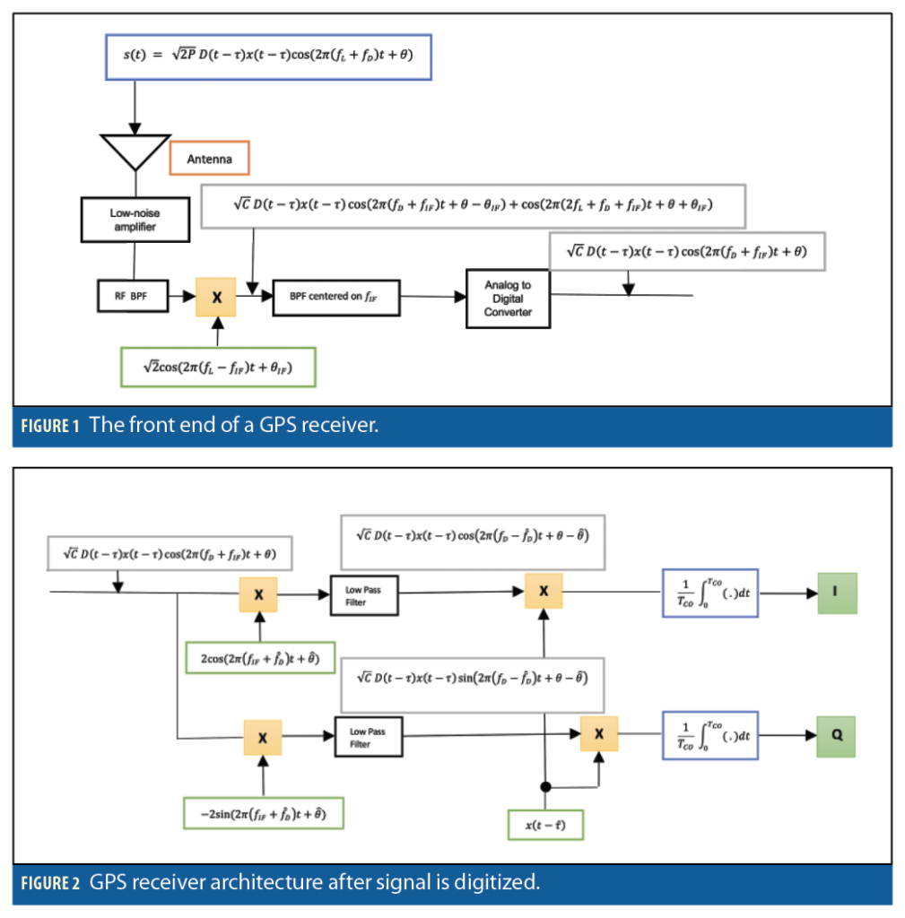
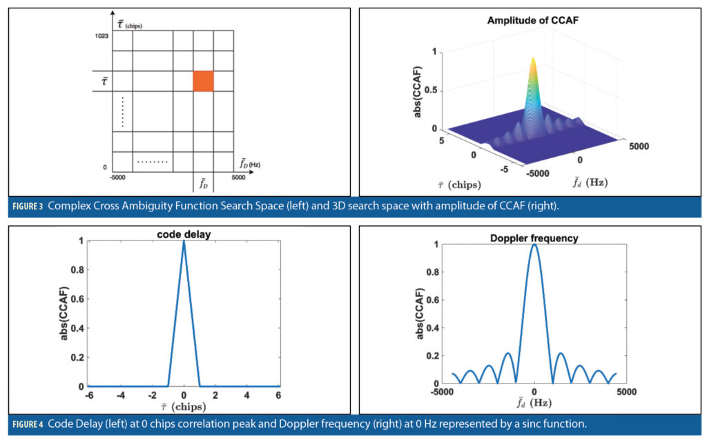
As shown in Figure 1, the GPS signal is received at a receiver’s antenna with code delay τ, Doppler fD, and carrier phase θ. The signal is then amplified, passed through a band pass filter, and then down converted to an intermediate frequency fIF by mixing with a locally generated mixing signal. It is then passed through a low pass filter to remove the high frequency components. The advantage of converting the signal to an intermediate frequency is it simplifies the subsequent stages, making filters easy to design and tune. The signal is then digitized and mixed again (Figure 2) with two locally generated replicas of the carrier signal fD, in-phase and quadrature, differing in phase by a quarter cycle, θ and θ+π/2. It is then passed through a low pass filter to remove the intermediate frequency, and finally mixed with a local replica of the PRN code with delay τ.
In-Phase and Quadrature Components
The in-phase I and quadrature Q components of an uncorrupted output signal (i.e., no spoofing or multipath) with amplitude √C are shown in Equations 1 and 2. When presented in complex form, as in Equation 3, the in-phase and quadrature components are the real and imaginary parts of the signal, respectively. The coherent integration time TCO can range from 1 to 20 milliseconds, the upper limit to avoid integration across boundaries of a GPS data bit D(t). Coherent integration is performed to reduce the effects of thermal noise.


Performing the integrals in Equations 1 and 2, Equation 3 can be expressed as

where+

and Tc is the duration of a single chip.
To simplify the notation, we define √C. Summing N component signals (i=1,…, N), we have

where g=(1,τ1,fD1,θ1,…,
N,τN,fDN,θN). For example, given the true satellite signal, a spoofed signal, and a single multipath signal, N=3.
Strictly, Equation 5 is true only for infinite length random codes. Finite length PRN codes like GPS L1 C/A, R(ξ) will have additional small, but non-zero, values outside the domain ξ∈(-Tc,Tc ). We ignore these for now but will address their impacts later.
CCAF Measurement Space
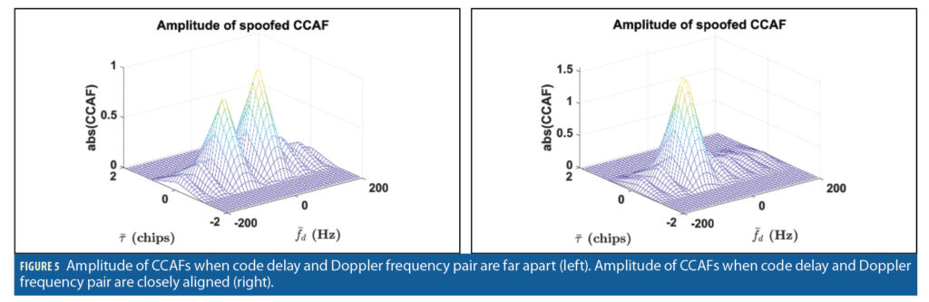
A Doppler frequency (fD) and code delay (τ) pair search sweep is done to correlate the incoming signal from satellites with a local replica. The measurement space is spanned by a two-dimensional grid across Doppler frequency fD and code delay τ. The carrier phase is held constant across the gird at an arbitrary value (for example at 0 or the punctual value retrieved from the loop; the actual number used does not matter). Each measurement then corresponds to a complex value SN (g|τ, fD), which is the CCAF.
When spoofing and multipath are not present, the magnitude of CCAF (i.e., the CAF) is visualized in Figure 3. The total number of cells in the measurement space is equal to the number of code phase bins times the number of Doppler bins.
When visualizing the CAF from the Doppler frequency point-of-view, the peak is represented by a sinc function with frequency 1/TCO; from the code delay view it is a triangle with base length of 2 chips (Figure 4). The coherent integration time affects the resolution of the Doppler frequency. It is generally preferred to have longer TCO for noise reduction reasons, but this will also require narrower Doppler bins because the sinc function itself becomes narrower. The software defined radio allows flexibility to change the Doppler bin widths. However, the code delay bins are determined by the sampling rate of the receiver.
Spoofing
When a spoofed signal is present and the code delays and Doppler frequencies of the signals are not closely aligned, two peaks are visible in the magnitude of the CCAF, ⎟⎟S2 (g|τ,fD)⎟⎟, as shown in Figure 5 (left). The two peaks merge if the code delays and Doppler frequencies are closely aligned, as shown in Figure 5 (right). The proposed idea is to decompose the CCAF of mixed signals into their constitutive parameters.
Particle Swarm Decomposition
Stacking the measurements from the grid space (τ,fD), the measurement model can be written as

where ν is the vector of measurement errors, including the effects of thermal noise and code cross-correlation. To decompose the N signals, we seek to obtain an estimate of the parameter vector, ĝ, that minimize the cost function.

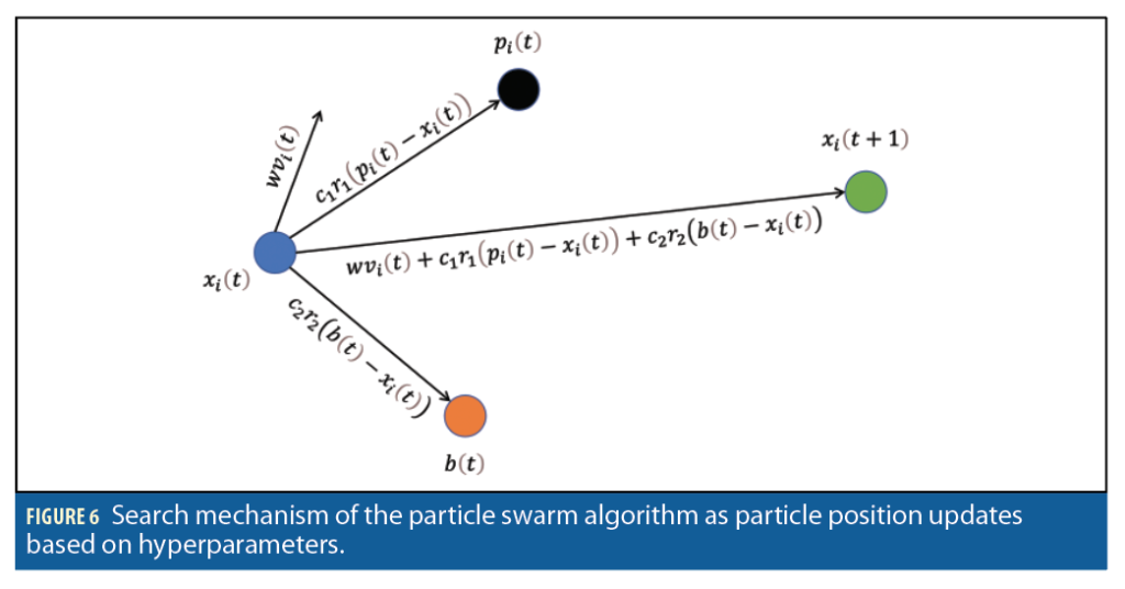
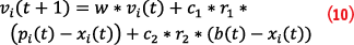
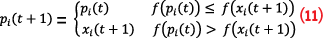
Unfortunately, due to the structure of SN the cost function is non-convex, and a global minimum cannot be obtained by standard gradient-based methods. In computational science, Particle Swarm Optimization (PSO) is an optimization algorithm that works by generating a population of “particles” randomly that are actually candidate solutions given upper and lower bounds. These particles are moved around in the N dimensional space based on their own best-known position pi and the entire population’s best-known position g as shown in Equations 9 and 10. When a particle finds a better position that minimizes the cost function better than the previous known position, pi gets updated based on Equation 11. If that particle’s position is best among all other particle positions (minimizes the cost function) b is updated based on Equation 12 and called the best global solution of the swarm.
A simple PSO algorithm is shown here:
Generate n number of particles generated randomly with “position” xi (t)∈X and “velocity”: vi (t)∈V
For each i=1,2,……,n particle


where:
r1,r2 are the uniformly distributed random number with Ν(μ,σ2)
w is the inertia coefficient
c1,c2 is the acceleration coefficient
pi (t) is the best local position
b(t) is the best global position
The PSO algorithm is applied to minimize the cost function J stated in Equation 8. The measurements z is in the form of CCAF, which is based on I and Qs and may be comprised of N signals, subtracts the CCAF(ĝ), SN (ĝ|τ,fD) based on the best global solution of the PSO algorithm is the cost function in this work, where ĝ=(â1,τˆ1,f ˆD1,θˆ1,…,âN,τˆN, f ˆDN,θˆN) are the estimates of the signals’ parameter.
Results
To evaluate the capability of the PSO algorithm in decomposing the multiple signals given the measurements, we decomposed the CCAF comprised of three signals, i.e., 12 parameters without any thermal noise and code cross correlation, and the results are:
Simulated Results
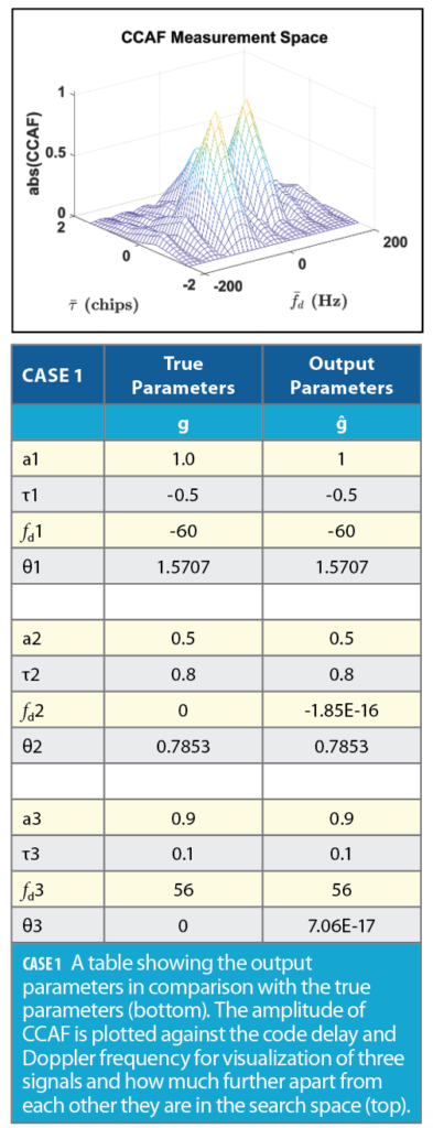
In Case 1, the CCAF is comprised of three signals in which the Doppler frequency and code delay pairs are closely aligned in the measurement space. The Particle Swarm Algorithm estimates and output of the signals’ parameters, ĝ are very close to the true parameters g as shown in Case 1 Table (bottom). For the purposes of visualization, CCAF magnitude is shown in Case 1 Figure (top) and all three signals can be identified by three distinct peaks.
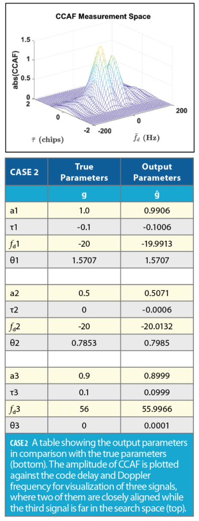
In Case 2, three signals are used in which the Doppler frequency and code delay pairs for the two signals are tightly aligned and the third signal is relatively far away in the CCAF measurement space. The PSO algorithm decomposed the signals and output their respective parameters ĝ as shown in the Case 2 Table (bottom) and are visualized in the Case 2 Figure (top). Note the two tightly aligned signals are merged and only one peak is identified when the CCAF magnitude is used.
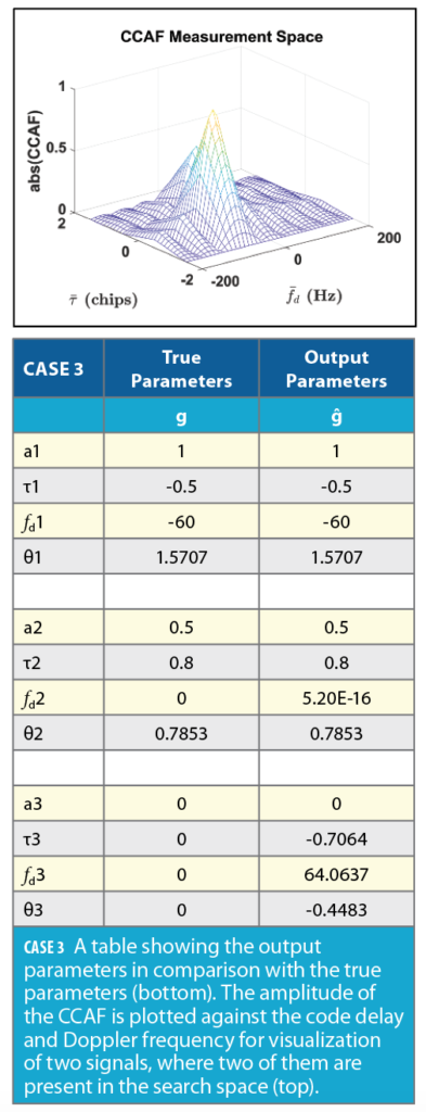
In Case 3, the input CCAF is comprised of two signals while the PSO algorithm searches for the three sets of signal parameters. This case is generated to evaluate the behavior of the algorithm in the scenario when there is only multipath signal present, and no spoofing. Because the algorithm is initialized in the same way as in Cases 1 and 2, the output is constrained to three signals. The third signal estimated by the algorithm has an amplitude of zero, implying the algorithm successfully identified there are only two signals present as shown in the Case 3 Table (bottom).
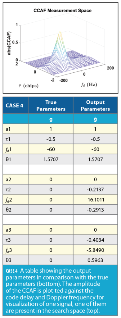
In Case 4, the input CCAF is comprised of only one signal, while the PSO algorithm tries to minimize the cost function for a CCAF comprised of the three signals. As shown in the Case 4 Table (bottom), two of the signals estimated by the algorithm have amplitudes of zero implying, again, the algorithm identified there is only one signal present with its parameters as the output ĝ.
Sensitivity Analysis
The PRN codes for the GPS L1 signal are transmitted at 1.023 Mega-chips per second (1,023 chips per millisecond) i.e.,1 code per millisecond, while the GNSS receiver usually has a faster sampling rate. The code is then distributed over the sampling rate of the receiver. To determine the precision of the algorithm, a sensitivity analysis is conducted next.
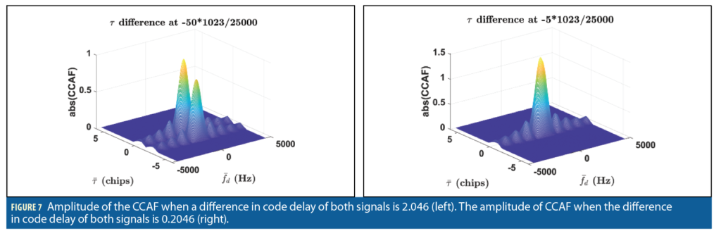
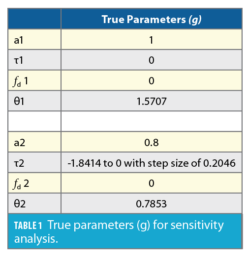
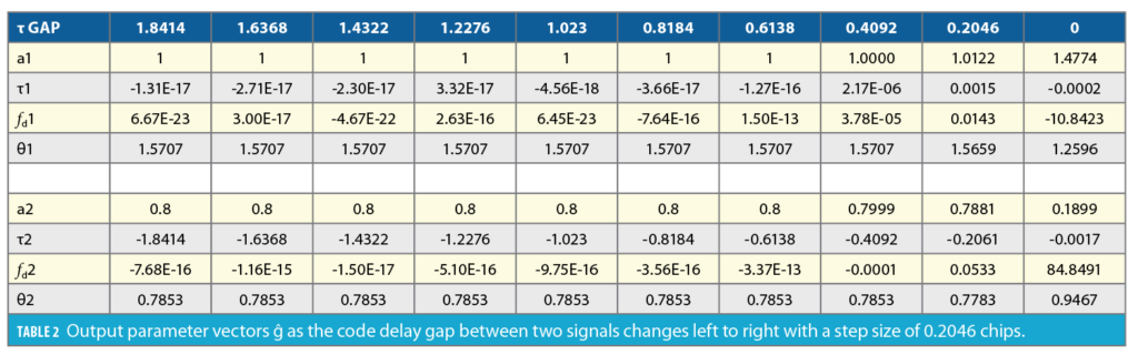
This analysis uses a 25 MHz sampling rate from the TEXBAT dataset. The samples per code is 25,000 and one chip contains 24 samples. The code delay search space consists of five chips with bin size of 0.0409 and Doppler bin ranges from -4500 Hz to 4500 Hz with bin size of 20 Hz. In each case, the candidate solution population is 1,000 and each case runs 100 iterations. We take a search space mixed with two CAFs as the two signals are further apart in the code delay and two peaks are sufficient to visualize the amplitude of CCAF as shown in Figure 7 (left). The CCAF with code delay at 0 chips is fixed and we change the second CCAF in code delay from -1.8414 to 0 with a step size of 0.2046. When the code delays for both signals are close in alignment, only one peak is detected (Figure 7, right).
The true parameters are shown in Table 1, while the output parameters’ decomposition results for each code delay gap is shown in Table 2. Until the code delay for both signals merges, the Particle Swarm Algorithm decomposes each CCAF into its respective output parameters very precisely.
Decomposition of the CCAF into the signals’ parameter vectors are shown in Table 2, as code delay gap between the two signals is reduced. When both signals are perfectly aligned in the CCAF evaluation space, there may be only one signal detected; the amplitude of the signal depends on the carrier phase of the signal. Note that when the Doppler frequency and code delay pair for both signals are in perfect alignment, there is no spoofing as the navigation solution for a spoofed signal is the same as the true signal. However, as soon as the spoofer tries to pull the location of the receiver off the truth, both CCAF are decomposed into the respective signals. If the amplitude for both is significant, spoofing is detected.
TEXBAT Dataset
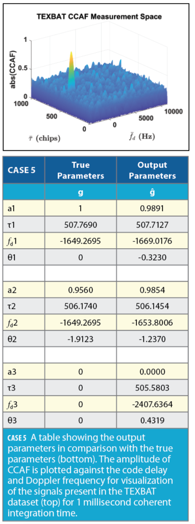
We have shown the capability of the Particle Swarm Algorithm to decompose CCAF made of up to N contributing signals and output the parameters vector ĝ without any noise and code cross-correlation present. To test the algorithm in a real scenario, we have taken an instant in the TEXBAT dataset that includes thermal noise and cross correlations. The measurement space for PRN 13 consists of 1,023 chips that are distributed over 25,000 samples, i.e., code delay bins, with Doppler frequency ranging from -3650 Hz to 11350 Hz with bin size of 10 Hz, a total of 1,501 bins. This can be seen in the figure in Case 5 (top), where two signal are present. The Particle Swarm algorithm searches for three signals, while the input CCAF has two prominent signals present. As shown in the Case 5 Table, the algorithm detects the signal parameters very near to the true parameters.
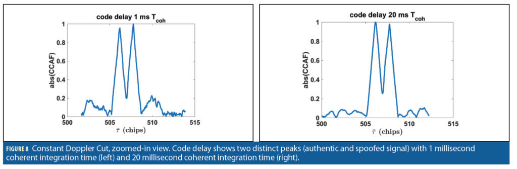
The two-signals detected by the algorithm are the authentic signal and the spoofing signal in the measurement space. The two signals are zoomed in and shown in Figure 8. The third signal that outputs by the PSD algorithm has zero amplitude, which represents there is no third signal present.
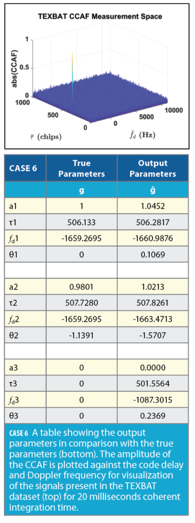
The noise floor as shown in Case 5 includes thermal noise. Cross correlations can be reduced by increasing the coherent integration time. In Case 6, the coherent integration time is 20 milliseconds because for GPS L1 C/A signal, the Navigation Data bit is 20 milliseconds long. The other advantage of using longer coherent integration time is the preciseness in code delay and Doppler frequency estimates from the Particle Swarm Decomposition Algorithm. The limit on coherent integration time can be disregarded if used in pilot signals.
The zoomed-in view of both Case 5 and Case 6 along a constant Doppler cut is shown in Figure 8. The noise floor in 20 milliseconds coherent integration time (Figure 8, right) is significantly lower than the 1 millisecond coherent integration time (Figure 8, left). Both results are normalized; one of the peaks represents an authentic signal and the other represents a spoofing signal. The peaks’ magnitudes also change with respect to each other when the coherent integration time changes from 1 millisecond to 20 milliseconds.
Spoofing Detection Monitor
Under normal circumstances, when spoofing is not present, the decomposed true signals will be geometrically consistent across all visible satellites but the decomposed multipath signals won’t. However, if spoofed signals are introduced, they also will be consistent across satellites. In this case, two independent decomposed signal sets (true and spoofed) will both be geometrically consistent across satellites. Our proposed basis for the spoofing detection is then to use an ‘inverse’ Receiver Autonomous Integrity Monitoring (RAIM) mechanism, where the existence of more than one consistent decomposed signal triggers a spoofing alarm.
Conclusion
In this article, we developed a method to decompose the CCAF into the N contributing signals by minimizing a cost function J and estimating the output parameter of vector ĝ. We have tested the algorithm in several challenging scenarios to determine its capability where the PSO algorithm searches for a greater number of signals than actually present in the CCAF measurement space. A sensitivity analysis has been performed on the characteristics of a GNSS receiver to demonstrate the capabilities of PSO in decomposing CCAF. We also demonstrated how PSO successfully decomposed the publicly available benchmarked spoofing dataset TEXBAT into two signals identifying their parameters.
Acknowledgment
This article is based on material presented in a technical paper at ION GNSS+ 2021, available at ion.org/publications/order-publications.cfm.
References
(1) T. E. Humphreys, B. M. Ledvina, M. L. Psiaki, B. W. O’Hanlon und P. M. Kintner, “Assessing the Spoofing Threat : Development of a Portable GPS Civilian Spoofer,” in Proceedings of the 21st International Technical Meeting of the Satellite Division of The Institute of Navigation (ION GNSS 2008), Savannah GA, 2008.
(2) M. Foucras, J. Leclère, C. Botteron, O. Julien, C. Macabiau, P.-A. Farine und B. Ekambi, “Study on the cross-correlation of GNSS signals and typical approximations,” in GPS Solutions, Springer Verlag, 2017.
(3) M. Pini, M. Fantino, A. Cavaleri, S. Ugazio und L. L. Presti, “Signal Quality Monitoring Applied to Spoofing Detection,” in Proceedings of the 24th International Technical Meeting of the Satellite Division of The Institute of Navigation (ION GNSS 2011), Portland OR, 2011.
(4) E. G. Manfredini, D. M. Akos, Y.-H. Chen, S. Lo, T. Walter und P. Enge, “Effective GPS Spoofing Detection Utilizing Metrics from Commercial Receivers,” in Proceedings of the 2018 International Technical Meeting of The Institute of Navigation, Reston, Virginia, 2018.
(5) T. Humphreys, J. Bhatti, D. Shepard und K. Wesson, “The Texas Spoofing Test Battery: Toward a Standard for Evaluating GPS Signal Authentication Techniques,” in Proceedings of the 25th International Technical Meeting of the Satellite Division of The Institute of Navigation (ION GNSS 2012), Nashville, TN, 2012.
(6) K. D. Wesson, D. P. Shepard, J. A. Bhatti und T. E. Humphreys, “An Evaluation of the Vestigial Signal Defense for Civil GPS Anti-Spoofing,” in Proceedings of the 24th International Technical Meeting of the Satellite Division of The Institute of Navigation (ION GNSS 2011), Portland, OR, 2011.
(7) H. Christopher,, B. O’Hanlon, A. Odeh, K. Shallberg und J. Flake, “Spoofing Detection in GNSS Receivers through CrossAmbiguity Function Monitoring,” in Proceedings of the 32nd International Technical Meeting of the Satellite Division of The Institute of Navigation (ION GNSS+ 2019), Miami, Florida, 2019.
Authors
Sahil Ahmed is currently a Ph.D. Candidate at the Navigation Laboratory in the Department of Mechanical and Aerospace Engineering, Illinois Institute of Technology (IIT). He also works as a Pre-Doctoral Researcher at Argonne National Laboratory. His research interest includes spoofing detection in GNSS receivers, software-defined radios (SDR), satellite communication, statistical signal processing, estimation and tracking, sensor fusion for autonomous systems, sense and avoid algorithms for unmanned aerial vehicles (UAV), machine learning and deep learning algorithms.
Dr. Samer Khanafseh is currently a research associate professor at Illinois Institute of Technology (IIT), Chicago. He received his Ph.D. degrees in Aerospace Engineering from IIT in 2008. Dr. Khanafseh has been involved in several aviation applications such as autonomous airborne refueling (AAR) of unmanned air vehicles, autonomous shipboard landing for the NUCAS and JPALS programs, and the Ground Based Augmentation System (GBAS). His research interests are focused on high accuracy and high integrity navigation algorithms, cycle ambiguity resolution, high integrity applications, fault monitoring, and robust estimation techniques. He is an associate editor of IEEE Transactions on Aerospace and Electronic Systems and was the recipient of the 2011 Institute of Navigation Early Achievement Award for his outstanding contributions to the integrity of carrier phase navigation systems.
Dr. Boris Pervan is a Professor of Mechanical and Aerospace Engineering at IIT, where he conducts research on advanced navigation systems. Prior to joining the faculty at IIT, he was a spacecraft mission analyst at Hughes Aircraft Company (now Boeing) and a postdoctoral research associate at Stanford University. Prof. Pervan received his B.S. from the University of Notre Dame, M.S. from the California Institute of Technology, and Ph.D. from Stanford University. He is an Associate Fellow of the AIAA, a Fellow of the Institute of Navigation (ION), and Editor-in-Chief of the ION journal NAVIGATION. He was the recipient of the IIT Sigma Xi Excellence in University Research Award (2011, 2002), Ralph Barnett Mechanical and Aerospace Dept. Outstanding Teaching Award (2009, 2002), Mechanical and Aerospace Dept. Excellence in Research Award (2007), University Excellence in Teaching Award (2005), IEEE Aerospace and Electronic Systems Society M. Barry Carlton Award (1999), RTCA William E. Jackson Award (1996), Guggenheim Fellowship (Caltech 1987), and Albert J. Zahm Prize in Aeronautics (Notre Dame 1986).


