
A comparison against classic models.
SHISHIR PRIYADARSHI, WAHYUDIN P. SYAM, ANDRÉS ABELARDO GARCÍA ROQUÉ, ALEJANDRO PÉREZ CONESA, GMV
GUILLAUME BUSCARLET, RAÜL ORÚS PÉREZ, MICKAEL DALL’ ORSO, EUROPEAN SPACE AGENCY (ESA)
Sun is the source of energy needed to ionize the Earth’s atmosphere, which is an envelope of different gases. It has 11-year solar cycles where solar activity varies from low, medium to high [1]. Solar activity is generally measured using the sunspot number as well as solar radio flux (also known as F10.7 cm Radio Flux). Sunspot numbers are between 0 to 30 during low solar activity, 30 to 60 during medium solar activity and > 60 with the ability to reach up to 300 during high solar activity.
With increasing solar activity, the Sun emits stronger particles as well as radiation toward Earth through solar events such as Coronal Mass Ejections (CMEs) and solar flares. Solar activity is also recognizable from the Sun’s appearance as well as a terrestrial phenomenon known as Aurora. Solar radiation ionizes the upper atmospheric layer of the Earth between 80 to 600 km. Because of the dominant presence of ions and electrons, this layer is widely known as the ionosphere. The ionosphere overlaps the upper atmosphere to the region where space begins. In its top atmospheric layer, the gases are cooked by solar radiation until they emit a few electrons. This process creates a sea of ions and electrons within the ionosphere, allowing the process of ionization and recombination to keep running seamlessly. The ionosphere is a highly variable medium. The ionospheric irregularities that are a direct threat for the trans-ionospheric radio communication spatially varies from a few centimetres to 1,000 kilometres on special scale.
Global infrastructure relies highly on a constellation of satellites (GNSS) that provides radio signals from space that transmit positioning and timing data to GNSS receivers [2-7]. These data are used for services like navigation, ranging, agriculture, tourism and transport. GNSS has global coverage, which is achieved using Europe’s Galileo, the U.S.’s Global Positioning System (GPS), Russia’s Global’naya Navigatsionnaya Sputnikovaya Sistema (GLONASS) and China’s BeiDou Navigation Satellite System.
The ionosphere is highly turbulent on a temporal scale where significant changes are observed from fractions of seconds, hours, days, seasons, years and solar cycles. It’s challenging to model a turbulent medium like the ionosphere. There are well established state-of-the-art ionospheric models, but when compared with real data, they significantly deviate from the actual ionospheric condition checked using GNSS observations. Today, several daily life services such as transport, weather, banking transition, tourism and navigation are highly reliant on the Total Electron Content (TEC) fluctuations derived along the navigation path of the GNSS signals. [8-12]. Improving GNSS positioning is challenging, and neural networks are one-of-a-kind robust tools that are useful for that purpose [13]. One of the methods in trend for characterization of the ionosphere and navigation is GNSS high frequency signal analysis [14]. TEC is a descriptive measure of the electron quantity between GNSS satellite and receiver, which is estimated using the time delay between two GNSS signal frequencies. Users cover a wide range of the ionosphere using a signal dual frequency receiver [15-16]. TEC is often represented in the multiples of TEC unit, where 1 TECU = 1016 el/m2, which is about 1.66 X 10⁻⁸ mol.m-2.
A few widely used and accepted empirical models such as Klobuchar [17], NeQuick-G [18] and International Reference Ionosphere (IRI) can produce the global morphology of the ionosphere during the geomagnetic quiet and disturbed days. Further, International GNSS Service (IGS) facilitates Global Ionospheric Maps (GIM) that records VTEC values of a spatial resolution of 2.5°×5°, and a 2-hour’s temporal resolution. These models and tools are good at reproducing the ionospheric geographic region as well as solar/geomagnetic activity dependent characterization, but still vary in error equivalent to 2-8 TECu for the same geographic locations during alike geomagnetic and solar activity condition. Geometrical effects are dominant at the lower latitude between satellite and receivers and add-on error to the ionospheric TEC estimation [19-20]. Physics based ionospheric models are often compromised in performance during low solar and geomagnetic activity [21-23]. These limitations and drawback of the ionospheric model and tools motivate the implementation of multi-layer machine learning (ML)-based models to improve the TEC forecasting accuracy and mitigate the degradation of the position accuracy induced by the ionosphere. Neural Network (NN) based TEC prediction models such as Han et al. [24], Ren et al. [25], Sivakrishna et al. [26], Shi et al. [27], Chen et al. [28], etc. are compromised as their predictive error increases with time and the global NN based TEC models fail to maintain regional accuracy in their forecast [29-30]. Another key aspect behind combining Multi-Layer Perceptron (MLP) + RNN, a hybrid approach, is the influence of other factors, such as space weather and geomagnetic indices, on the variations in the nonstationary patterns of ionospheric TEC.
This study compares the performance of the HARMONY (macHine leARning to MOdel gNss sYstems) ionospheric demonstrator (MLD-IONO) to the NeQuick-G, Klobuchar ionospheric models and GIM maps) during the high solar activity period at three different geographic locations.
Data and Methodology
Machine Learning Ionospheric Model (MLD: ML IONO Demonstrator)
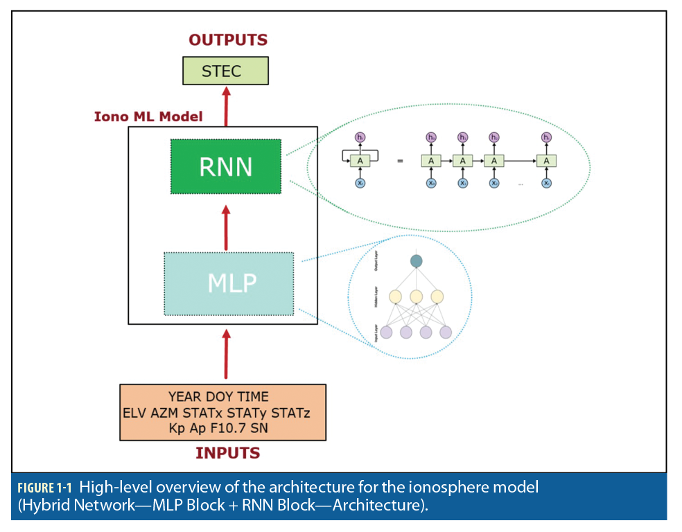
Using a combination of Multi-Layer Perceptron (MLP) and a Long-Short Term Memory (LSTM) based recurrent neural network (RNN) (Figure 1-1) a ML ionospheric model has been trained, which can nowcast and forecast the ionosphere over Europe and North Africa latitudes. While this abstraction seems intuitive and using the RNN can be considered because of its known capacity to process inputs of any length as well as to better “remember” the patterns along a time sequence, the applicability and benefits of this architecture is already determined during model validation. To assess the feasibility of this hybrid architecture, we considered a traditional RNN as well as a GRU and a LSTM. Model training used RINEX observation and navigation files along with the solar and geomagnetic indices, which were taken from public archives. The combination of MLP and LSTM keeps the good regression performance while providing additional capability to best exploit the information along the time axis. The final model has been tested and validated against real observations and along with state-of-the-art single frequency ionospheric models such as NeQuick-G and Klobuchar.
NeQuick-G is a three-dimensional time varying electron density model that predicts monthly mean electron density using the analytical profiles, geographic location and solar activity condition. Klobuchar is a simple structure model as it considers the ionosphere as a single layer at the height of 350 km.
Ionospheric correction coefficients, which are eight in numbers, are transmitted by the satellites in the navigation message on a daily basis for GPS and are used to calculate the ionospheric delay. The Klobuchar model uses a 5 previous days average of solar flux due to which Klobuchar coefficients are updated once a day for GPS. These coefficients are based on the day of year (DOY).
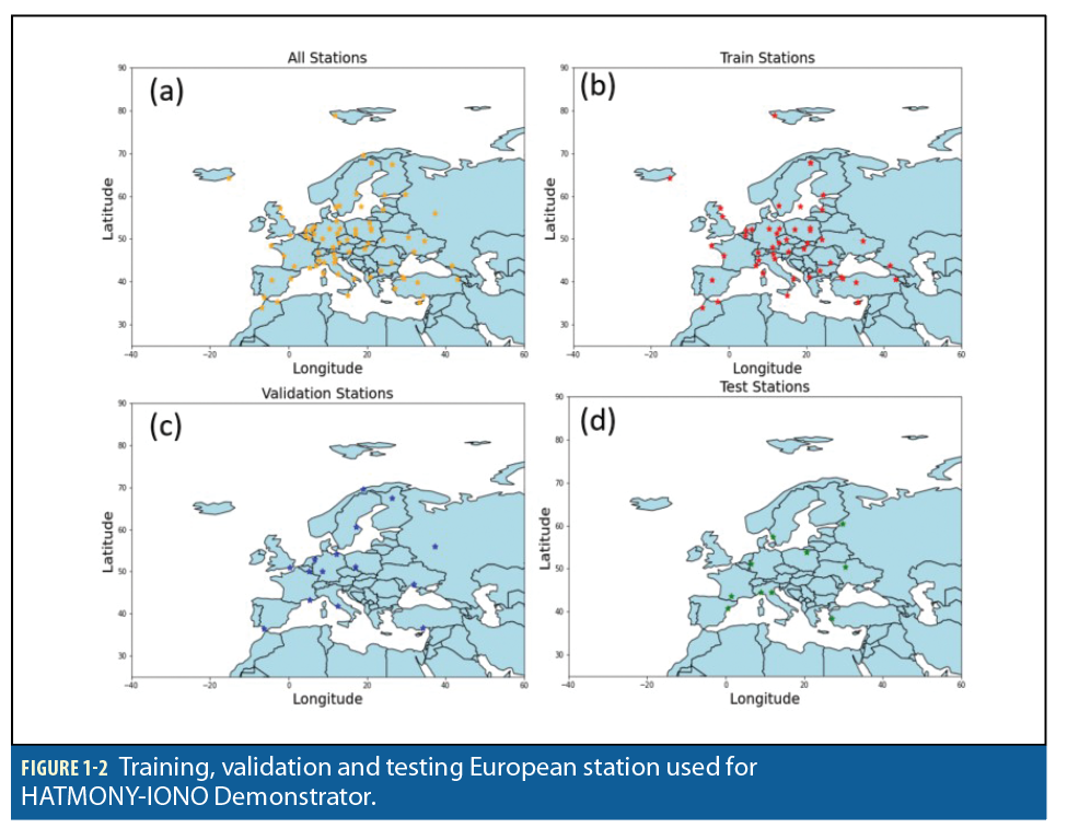
Figure 1-2 shows the location of stations considered for: (a) Ionosphere model implementation, (b) Training phase, (c) Validation phase, and (d) Training, testing and validation of the ionosphere model. Different experiments were performed using different configurations for the MLP architecture. Best hyperparameters were an MLP with 5 layers and an initial layer with 512 neurons and ReLU as the activation function, learning rate equal to 1e-5 and batch size of 184.
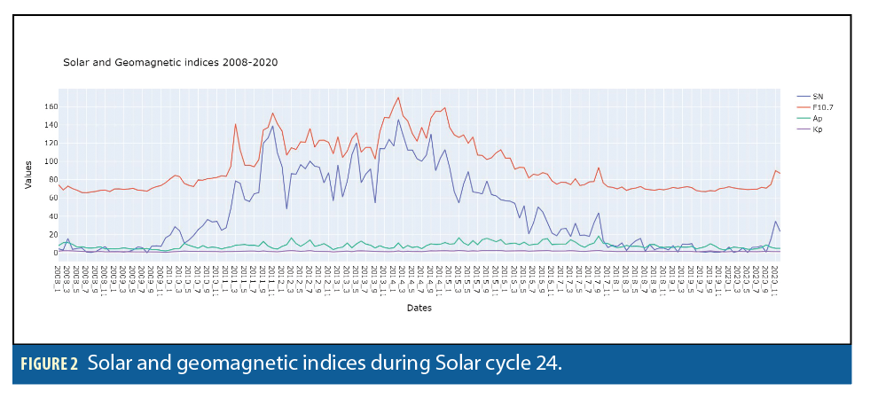
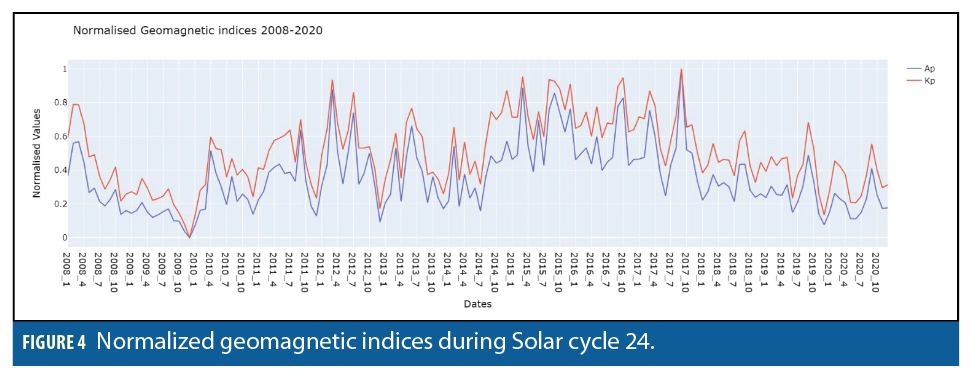
Because we decided to consider Solar cycle 24 as the period to collect our data and perform the analysis, we had to first understand how this solar cycle has evolved by looking at its periodicity. As illustrated in Figure 2, it is possible to distinguish an ascending and descending phase along the period from 2008 to 2020 characterized by high solar activity (high values of the F10.7 and SN parameters) during the ascending phase and lower solar activity during the descending phase.
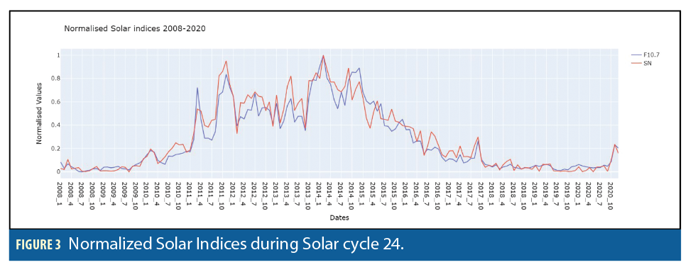
It is worth noting that even in Figure 2, both geomagnetic and solar indices are represented, and the two groups of indices have a different scale and periodicity. With a closer look at their normalized evolution along the same time span (Figures 3 and 4), it is easier to distinguish how the solar parameters describe a clear ascending-descending cycle reaching peak during 2014, while geomagnetic parameters do not fluctuate following the same pattern.
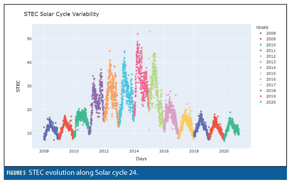
Solar and geomagnetic parameters have been considered because of their influence on ionosphere behavior. When plotting the evolution of the STEC values (Figure 5), it is possible to see three different timescale patterns:
1. SOLAR CYCLE VARIABILITY: This pattern matches one previously defined by the variation of the solar parameters. In this case, STEC values rise according to the solar cycle ascending phase to later decrease on the descending phase. Similarly, STEC peak values were obtained in 2014. Each STEC value has been computed as the mean of all the STEC values recorded for all the stations available for that particular point in time.
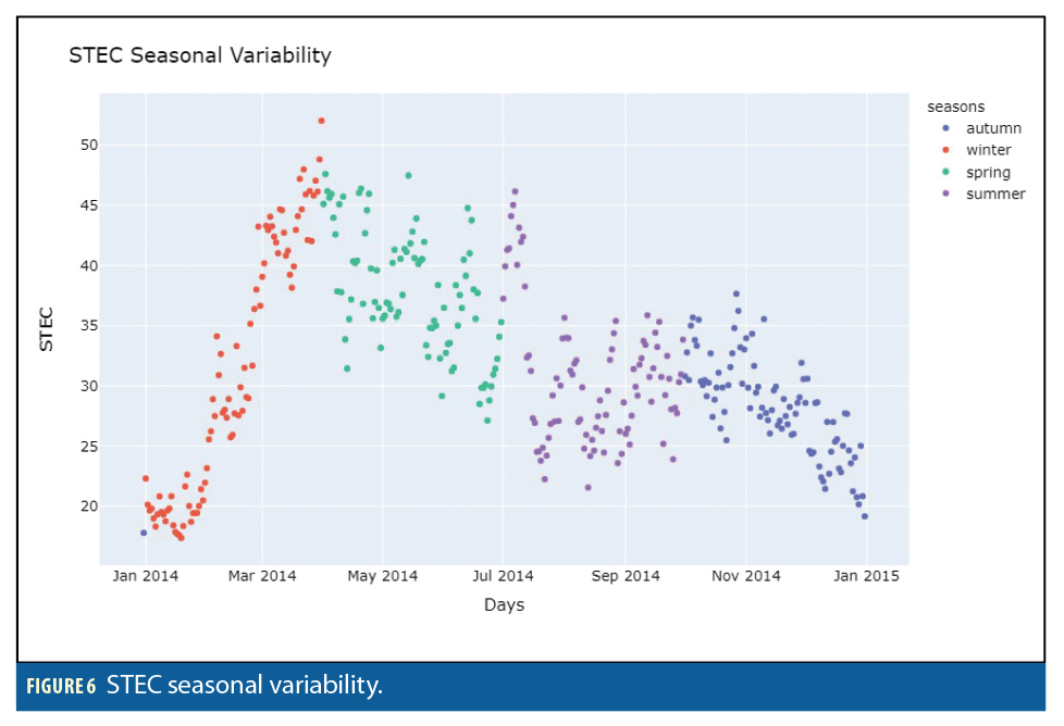
2. SEASONAL VARIABILITY: While you need to analyze the STEC along multiple years to visualize the first-time scale, it is also possible to find a second time pattern associated to the seasonal variability (Figure 6). Along each year, the STEC values show a steep increase during winter that progressively decrease during spring, summer and autumn. It is worth noting that by the end of spring and the start of summer, the STEC value shows a second smaller peak. As before, each STEC value is the averaged STEC of all available stations for that given point in time.
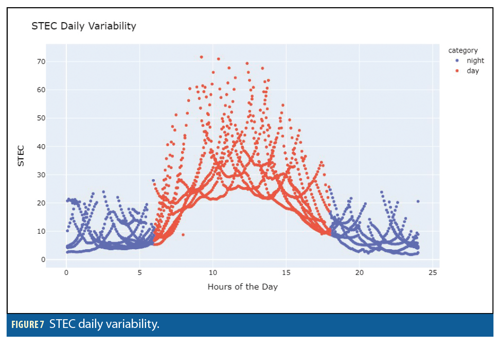
3. DAILY VARIABILITY: The third
timescale, which influences STEC behavior, is associated with diurnal and nocturnal cycle. As seen in Figure 7, STEC values tend to reach peak during midday hours while remaining lower at night (early morning and late evening). STEC values represented in this plot are values of one fixed station and fixed date.
Results and Discussion
Comparison of the MLD STEC/VTEC forecast to the known real STEC and GIS VTEC
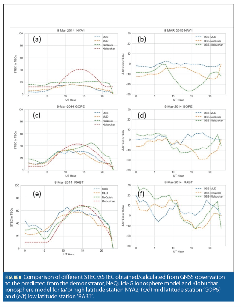
High solar activity conditions are interesting to model at low-, mid-, and high-latitude regions due to the high solar indices that control the ionospheric instabilities formation dynamics. The presented space weather scenario covers the execution of the ML model for ionosphere modeling during a high ionospheric activity condition on March 8, 2014 for the low-, mid- and high- latitude stations Rabat Morocco (RABT00MAR), Ondrejov, Czechia (GOP600CZE), and Ny Alesund, Norway (NYA200NOR) respectively.
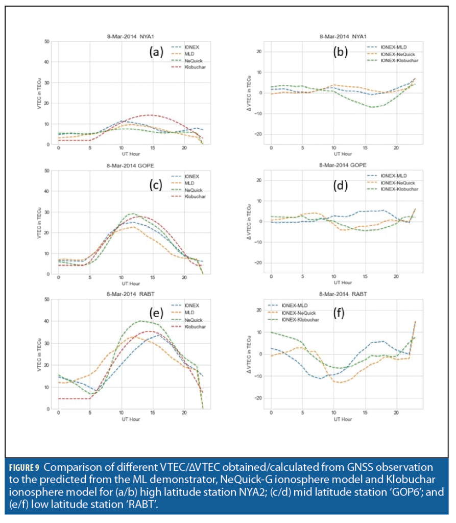
The STEC and ∆STEC comparison at the three stations during high ionospheric activity that day (Figure 8) shows the MLD STEC output was much better than the NeQuick-G and Klobuchar modeled STEC at all three stations. Figures 8 and 9 demonstrate that MLD STEC and VTEC are close to the STEC observation and IONEX (IONosphere map Exchange format) VTEC whereas the MLD difference to the real data scenario seems to vary around zero, which means they have minimal deviation from the real data in comparison to the NeQuick-G and Klobuchar ionospheric model produced STEC/VTEC. IONEX format developed to exchange, compare or combine TEC maps. IONEX format supports the exchange of two- and three-dimensional TEC maps given on a geographic grid.
In this particular case, MLD VTEC performed better than NeQuick-G-G. The Klobuchar-produced VTEC matches quite close to the NeQuick-G VTEC (Figure 9).
Comparison of R2 STEC/VTEC
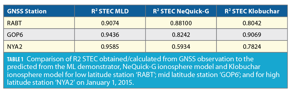
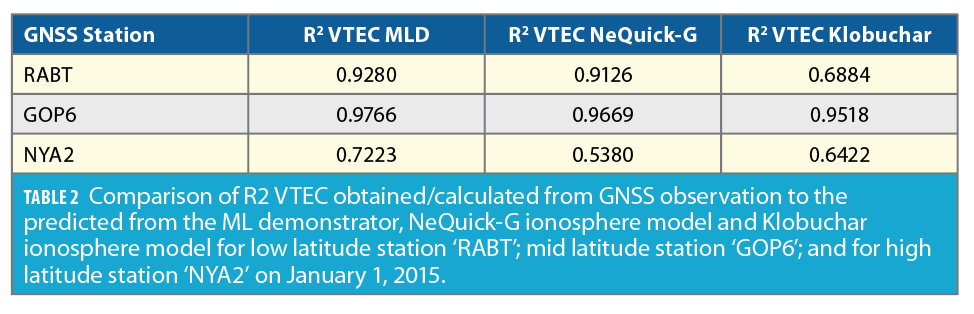
Tables 1 and 2 show the MLD KPIs are better than the two models used at mid and high latitudes, however they are comparable to NeQuick-G at low latitude.
The correlation table shows the MLD performance was better overall (Tables 1 and 2) NeQuick-G’s performance was good for mid and high latitude, whereas Klobuchar VTEC has high value at mid- and low-latitude stations on March 8, 2014.
MLD KPIs were best for STEC at all latitudes, for VTEC MLD is comparable to NeQuick-G at the station ‘GOPE.’ At the ‘RABT’ station, all three model outputs are comparable and within acceptable RMSE range on March 8, 2014. The NeQuick-G ionospheric model’s forecast of STEC and VTEC was executed for all three stations. We present here STEC data at a 20 to 40 degree elevation angle. The same input parameters have been used for shorting data for ML model predictions, as well as the NeQuick-G model. For VTEC, we provided ionospheric pierce point latitude and longitude at a shell height of 350 km.
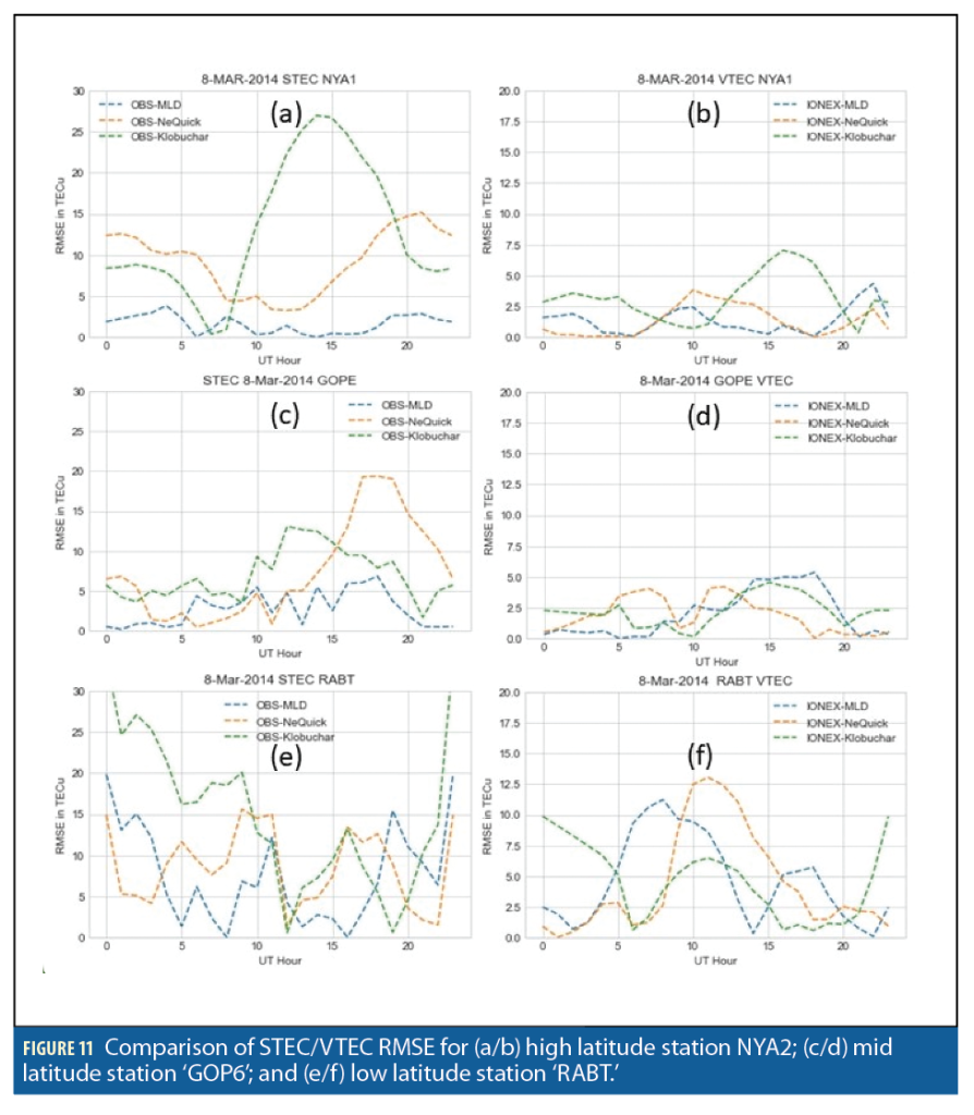
Comparison of NeQuick-G/Klobuchar Ionosphere Model and STEC/VTEC predictions
The NeQuick-G-G/Klobuchar ionospheric model’s forecast of STEC and VTEC was executed for all three stations. We present STEC data at a 20 to 40 degree elevation angle. The same input parameters were used for shorting data for the ML model predictions, as well as the Klobuchar model. For VTEC, we provided ionospheric pierce point latitude and longitude at a shell height of 350 km (Figures 11 and 12).
GOP6 and NYA2 stations had the best MLD STEC and VTEC performances. But it was likely redundant to the NeQuick-G and Klobuchar for the ‘RABT’ station.
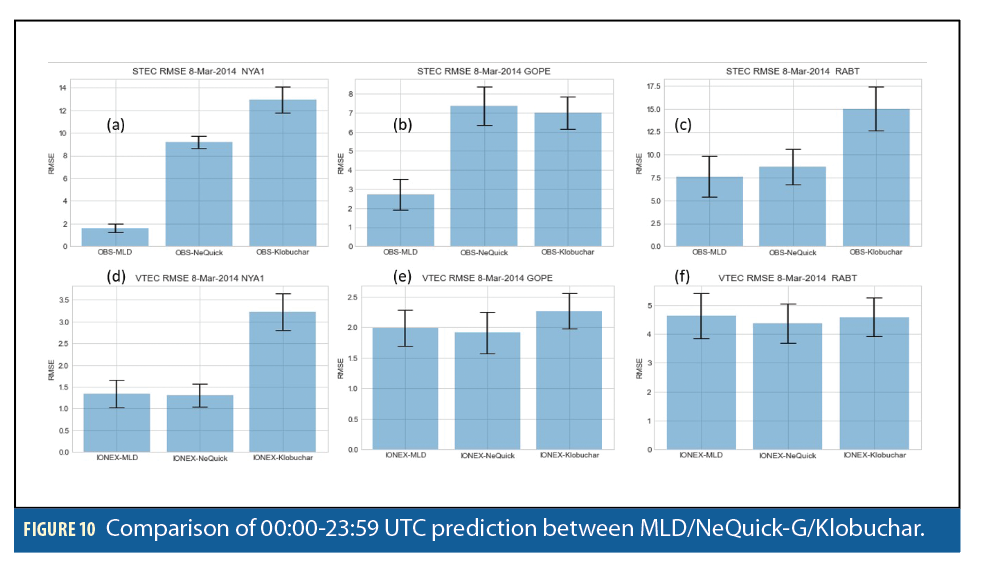
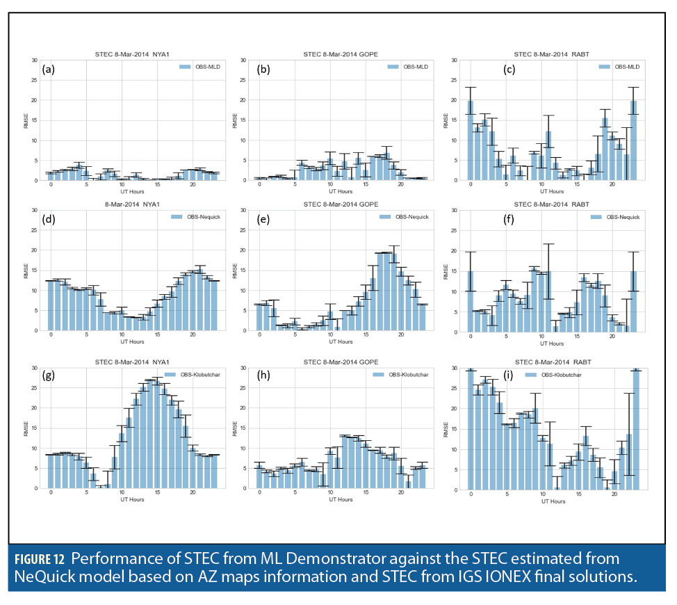
MLD KPI’s comparison to the NeQuick-G/Klobuchar ionospheric model
The accuracy of the MLD-IONO model was tested using well established ionospheric models Klobuchar and NeQuick-G during low, medium and high solar activity. Overall, for high and mid latitude, MLD-IONO KPIs are lower than the OBS-NeQuick-G and OBS-Klobuchar KPIs. However, due to the lack of enough training data at the low latitude, MLD-IONO, performance is comparable to NeQuick-G and is better than the Klobuchar ionospheric model (Figures 11 and 12).
Summary, conclusion and future works
The HARMONY MLD-IONO is intended to overcome the limitations of simulations based on a GNSS macro-model through the implementation of a ML model that models a GNSS system, providing better performances once trained to predict its behavior. Apart from a performance boost, the ML demonstrator could also leverage the use of previously unused data sources, providing knowledge of hidden phenomena and unknown relations. It was also found that the ML model predicted VTEC more realistically than NeQuick-G. Klobuchar forecasted VTEC matches quite close to NeQuick-G. The performance of the developed ionospheric machine learning model is highly dependent on solar and geomagnetic activity and the receiver location.
In general, with all the stations, demonstrator performance was within the acceptable KPIs range. In the future, we would like to extend this study by ingesting ground magnetometer data to see any possible connection between a ground induced current and the ionospheric variability. Our future activities will focus on developing new compact tools and Sun-Earth relationships based on space weather models suitable to mimic/forecast the extreme solar events that are a threat to the power grid and services that rely on it.
Acknowledgments
This work was supported by the European Space Agency NAVISP program and funded under the activity EL1-035 ter: “Machine Learning to Model GNSS Systems.”
References
(1) Nicola, S., Antonio, B. (2022). The Planetary Theory of Solar Activity Variability: A Review, Frontiers in Astronomy and Space Sciences, 9(2022), https://doi.org/10.3389/fspas.2022.937930
(2) Morton, Y., Taylor, S., Wang, J., Jiao, Y., Pelgrum, W. (2013). In L band ionosphere scintillation impact on GNSS receivers. In Proceedings of the IEEE Radio Science Meeting (USNC-URSI NRSM), US National Committee of URSI National, Boulder, CT, USA, 9–12 January 2013, 1.
(3) Chen, X., Dovis, F., Peng, S., & Morton, Y. (2013). Comparative studies of GPS multipath mitigation methods performance. IEEE Transactions on Aerospace and Electronic Systems, 49(3), 1555–1568.
(4) Ghafoori, F., Skone, S., (2015). Impact of equatorial ionospheric irregularities on GNSS receivers using real and synthetic scintillation signals. Rad. Sci., 50, 294–317.
(5) Kintner, P., Ledvina, B., De Paula, E. (2007). GPS and ionospheric scintillations. Space Weather 5, 83–104.
(6) Jacobsen, K.S., Dahnn, M. (2014). Statistics of ionospheric disturbances and their correlation with GNSS positioning errors at high latitudes. J. Space Weather Space Clim., 4, A27.
(7) Tiwari, R., Strangeways, H.J., Tiwari, S., Ahemad, A. (2013), Investigation of ionospheric irregularities and scintillation using TEC in high latitude. Adv. Space Res., 52, 1111–1124.
(8) Tang, L., Yang, X., Kan, Z., Li, Q. (2015). Lane-level road information mining from vehicle GPS trajectories based on naïve bayesian classification. ISPRS Int. J. Geo-Inf., 4, 2660–2680.
(9) Xie, X., Wong, K.B.-Y., Aghajan, H., Veelaert, P., Philips, W. (2015). Inferring directed road networks from GPS traces by track alignment. ISPRS Int. J. Geo-Inf., 4, 2446–2471.
(10) Li, J., Zhang, Y., Wang, X., Qin, Q., Wei, Z., Li, J. (2016). Application of GPS trajectory data for investigating the interaction between human activity and landscape pattern: A case study of the Lijiang River Basin, China. ISPRS Int. J. Geo-Inf., 5, 104.
(11) Ranacher, P., Brunauer, R., van der Spek, S., Reich, S. (2016). What is an appropriate temporal sampling rate to record floating car data with a GPS? ISPRS Int. J. Geo-Inf., 5, 1.
(12) Wu, T., Xiang, L., Gong, J. (2016). Updating Road networks by local renewal from GPS trajectories. ISPRS Int. J. Geo-Inf., 5, 163.
(13) Kanhere, A. V., Gupta, S., Shetty, A., and Gao, G. (2022). Improving GNSS Positioning Using Neural-Network-Based Corrections. NAVIGATION: Journal of the Institute of Navigation, 69 (4) navi.548. https://doi.org/10.33012/navi.548
(14) Baumgarten, Y., Psiaki, M.L.,and Hysell, D.L. (2022). Navigation and Ionosphere Characterization Using High-Frequency Signals: A Performance Analysis. NAVIGATION: Journal of the Institute of Navigation, 69(4) navi.546. https://doi.org/10.33012/navi.546
(15) Farzaneh, S., Forootan, E. (2020). A Least Squares Solution to Regionalize VTEC Estimates for Positioning Applications. Remote Sens., 12, 3545. https://doi.org/10.3390/rs12213545
(16) Ya’acob, N., Abdullah, M., Ismail, M. (2010). GPS Total Electron Content (TEC) Prediction at Ionosphere Layer over the Equatorial Region. In: Bouras, C., editor. Trends in Telecommunications Technologies [Internet]. London: IntechOpen; 2010 [cited 2022 Nov 25]. Available from: https://www.intechopen.com/chapters/9691. https://doi.org/10.5772/8474
(17) Klobuchar, J. (1987). Ionospheric Time-Delay Algorithms for Single-Frequency GPS Users. IEEE Transactions on Aerospace and Electronic Systems, 3, 325-331.
(18) Prieto-Cerdeira, R., Orús-Pérez, R., Breeuwer, E., Lucas-Rodríguez, R., and Falcone, M. (2014). ‘Innovation: The European Way. Performance of the Galileo Single-Frequency Ionospheric Correction During In-Orbit Validation’. In: GPSworld 25.6, 53–58. Categories: FundamentalsGNSS Measurements Modelling.
(19) Singleton, D.G. (1970). Dependence of satellite scintillations on zenith angle and azimuth. J. Atmos. Terr. Phys. 32, 5, 789-803, https://doi.org/10.1016/0021-9169 (70)90029-2
(20) Priyadarshi, S., Wernik, A.W. (2013). Variation of the ionospheric scintillation index with elevation angle of the transmitter. Acta Geophys. 61, 1279–1288. https://doi.org/10.2478/s11600-013-0123-3
(21) Priyadarshi, S. (2015a). A Review of Ionospheric Scintillation Models. Surv Geophys, 36, 295–324. https://doi.org/10.1007/s10712-015-9319-1
(22) Priyadarshi, S. (2015b). Ionospheric scintillation modeling for high- and mid-latitude using B-spline technique. Astrophys Space Sci., 359, 12. https://doi.org/10.1007/s10509-015-2461-x
(23) Priyadarshi, S., Zhang, Q.-H., Ma, Y.-Z., Wang, Y., and Xing, Z.-Y. (2016). Observations and modeling of ionospheric scintillations at South Pole during six X-class solar flares in 2013. J. Geophys. Res. Space Physics, 121, 5737– 5751. https://doi.org/10.1002/2016JA022833
(24) Han, Y., Wang, L., Fu, W., Zhou, H., Li, T., and Chen, R. (2021). Machine Learning-Based Short-Term GPS TEC Forecasting During High Solar Activity and Magnetic Storm Periods. IEEE Journal of Selected Topics in Applied Earth Observations and Remote Sensing, 15,115-126. https://doi.org/10.1109/JSTARS.2021.3132049
(25) Ren, X., Yang, P., Liu, H., Chen, J., Liu, W. (2022). Deep Learning for Global Ionospheric TEC Forecasting: Different Approaches and Validation. Space Weather, 20, e2021SW003011.
(26) Sivakrishna, K., Venkata, R.D., Sivavaraprasad, G. (2022). A Bidirectional Deep-Learning Algorithm to Forecast Regional Ionospheric TEC Maps. IEEE J. Sel. Top. Appl. Earth Obs. Remote Sens., 15, 4531–4543.
(27) Shi, S., Zhang, K.,Wu, S., Shi, J., Hu, A., Wu, H., Li, Y. (2022). An Investigation of Ionospheric TEC Prediction Maps Over China Using Bidirectional Long Short-Term Memory Method. Space Weather, 20, e2022SW003103.
(28) Chen, Z., Liao, W., Li, H., Wang, J., Deng, X., Hong, S. (2022) Prediction of Global Ionospheric TEC Based on Deep Learning. Space Weather, 20, e2021SW002854.
(29) Priyadarshi, S., Syam, W., Roqué, A.A.G., Conesa, A.P., Buscarlet, G., Pérez, R.O. and Orso, M.D. (2023, January). Machine Learning-based ionospheric modelling performance during high ionospheric activity. In Proceedings of the 2023 International Technical Meeting of The Institute of Navigation (ION ITM 2023) (pp. 950-965).
(30) Syam, W.P., Scott, D., Perez-Conesa, A., Rodriguez, I., Lechuga, M.L., Martinez, E.J. and Ioannidis, R.T. (2023). Navigating Emergencies with a Low-RF CARS. Inside GNSS, 18, 1, p.40.
Authors
Shishir Priyadarshi obtained his Ph.D. in Space Physics from the Space Research Centre, Poland, in 2014. Thereafter, he held various international postdoctoral, visiting scientist and adjunct faculty positions between 2014 and 2021. Subsequently, he joined GMV as a Machine Learning Engineer in 2022.
Wahyudin P. Syam holds a Ph.D. in geometrical measurement and uncertainty analysis from Politecnico di Milano in Milan, Italy. He joined GMV in February 2021. At GMV, he is involved in several ESA projects related to GNSS fingerprinting and IGS orbit and clock-bias corrections.
Andrés García holds a bachelor’s degree in computer engineering as well as a master’s degree in data science and engineering. For two years he has worked in GMV Innovating Solutions as a big data engineer and then changed to a machine learning engineer position.
Alejandro Pérez Conesa received his B.Sc. degree in Computer Engineering and his B.Sc. and M.Sc. degrees in Telecommunication Engineering from the Universitat Autònoma de Barcelona (UAB) in 2018, 2019 and 2020, respectively. He is currently working as Project Manager for GMV and as Adjunct Professor at UAB.
Guillaume Buscarlet graduated from Supaero (ENSAE) Toulouse, France, in 1997, worked at Thales Alenia Space, Toulouse, France in Navigation (EGNOS) and Telecom (IRT Saint-Exupery, Digital P/L). Since 2020, he has worked at ESA (EGNOS Project Office) as a SBAS System Performance Engineer for EGNOS.
Raul Orus Perez received a Ph.D. in Aerospace Science and Technology from the gAGE/UPC research group of the Technical University of Catalonia (UPC) in 2005. Since 2010, he has worked at ESA/ESTEC as a Propagation Engineer (radio-wave propagation in troposphere and ionosphere).
Mickael Dall’Orso received his M.Sc degree from ISAE-ENSICA (French Institute of Aeronautics and Space) in 2010, Toulouse, France. He worked until 2018 in SBAS algorithms and performances (EGNOS, KASS) at Thales Alenia Space in Toulouse. He is currently an EGNOS System Performance Engineer at ESA’s EGNOS Project Office in Toulouse.


