
A new approach to achieving the safety needed for levels 3 and higher of autonomy builds on a thorough mathematical framework to support safety analysis, while delivering very tight position bounds.
The autonomous car represents the epitome of safety-critical autonomous functionality. The most important reason to build autonomous cars is to lower the rate of injury and death on roads around the planet. Policy makers and the automotive industry firmly believe that autonomy can dramatically reduce this toll, but it depends on our ability to engineer truly safe autonomous functionality into the car.
As we move towards this level of autonomy, we see more and more sensors built into vehicles. Radar, LiDAR, vision and ultrasonic sensors are all in the mix, offering relative positioning capability. In other words, they can tell us how far away other objects are from the vehicle, and, by sensing the distance from landmarks, they can also be used to position it relative to the reference frame defined by these landmarks. For some use cases, however, a truly absolute positioning sensor is needed, and this is where GNSS or, more typically, GNSS fused with inertial sensors comes into the picture. Examples of such use cases include:
• Determining that the vehicle has entered a highway where it is safe to engage autonomy features;
• Determining longitudinal location of the vehicle with respect to curves and other features of the roadway as an aid to interpreting images and other sensor data;
• Determining position and velocity of the vehicle to calibrate other sensors
As an ambition we could also hope to employ GNSS/INS with other sensors for lane identification.
What is needed for level 3 to 4 autonomy is a system of positioning that provides dynamic error bounds at the level of a few meters or less for a high proportion of the time under challenging highway conditions. Ultimately, for levels 4 and 5, we will need this even deep inside urban areas. For these systems, the targeted rate of dangerous positioning errors is expected to be lower than one occurrence in 10 million hours of driving. Clearly, this is challenging to prove by test, and that means that the technological solution must be open to the most rigorous examination by experts.
Aviation vs Automotive
To employ GNSS receivers in safety-critical applications, it is necessary to compute safe bounds on the position error, and this is notoriously difficult for GNSS. The one exception is in aviation navigation that has developed so-called integrity monitoring concepts for about two decades now. These concepts are the outcome of a particularly detailed understanding of the errors and faults affecting GNSS systems as well as of a thorough mathematical framework to ensure the appropriate level of bounding.
A key element of any integrity monitoring concept is the notion of protection level (PL). The PL represents a bound on the position error that ensures that the system is safe when it is below the required alert limit. Several mechanisms have been defined in the context of aviation to compute a rigorous and safe PL. They are dependent upon the type of augmentation used (SBAS, GBAS, ABAS), but in the end, they all aim at solving the same PL equation. These standardized integrity algorithms have usually been defined in the context of single frequency single GNSS and considering the reception conditions of a flying aircraft.
Recently, however, significant advances have been made to account for the availability of multiple GNSS frequencies and multiple GNSS constellations. Dual frequency provides the capability of removing the ionospheric delay affecting measurements while multiple GNSS constellations improve the measurement redundancy and thus the fault detection and exclusion capability, as well as the PL magnitude. A good example of these new integrity algorithms is the development of advanced RAIM (ARAIM) that only relies on a minimal external message providing information on satellite and GNSS constellation failures.
For non-aviation applications, ARAIM is an interesting integrity algorithm because it is now well understood and has been rigorously investigated. Since it relies on a receiver-autonomous detection of faults, it is also well suited when not all GNSS fault sources are addressed by other augmentation systems (as is the case in the SBAS and GBAS frameworks). It is also important for applications that require very small time-to-alert (TTA) that would not allow for detection by a separate system.
However, transforming ARAIM for the automotive application is not a straightforward operation. The use of ionosphere-free (IF) measurements is known to increase the magnitude of errors that are uncorrelated between frequencies, such as thermal noise, multipath, or some biases. In a typical road environment, this is likely to give large position uncertainties.
Besides, aviation receivers typically phase-smooth their pseudorange over 100 seconds to reduce the magnitude of noise and multipath. This approach cannot be used by automotive users because it is unlikely that carrier-phase tracking can be maintained reliably over long periods of time due to the environment.
Finally, most of the foreseen automotive applications are expected to have alert limits and TTA specifications that are more stringent than in aviation (typically alert limit in the range of 0.5 to 10 m and TTA around 1 sec) without necessarily requiring a less stringent integrity risk. This means that the typical magnitude of ARAIM PL might be too large.
Because of these considerations, it appeared natural to make use of time-filtering to improve the performance of ARAIM in terrestrial conditions. Moreover, the desire to complement GNSS with other sensors such as inertial measurement units (IMUs) or wheel speed sensors (WSSs) led to the consideration of a version of ARAIM that is built upon an extended Kalman filter (EKF) rather than a weighted least square (WLS) snapshot analysis. Aviation has been using time-filtering and IMU integration for some years now.
Instead of using phase-smoothed pseudorange measurements, the EKF can benefit directly from the phase measurements. Finally, further reduction in the magnitude of the PL can be expected by using corrections, either in the form of PPP or PPP-RTK, although the understanding of these corrections (uncertainty, fault modes) then becomes critical. This version of ARAIM will be referred to as EKF-ARAIM here.
EKF-ARAIM (and a version of it referred to as Batch-ARAIM) has been the topic of many publications. However, there are still several problems. Two examples are:
• Because the EKF uses time-series of measurements, the position overbounding mechanism has to account for errors that are time-correlated. The most recent research on this topic has led to a new overbounding solution, namely frequency domain overbounding, but the rigorous use of this method is only valid when some strict assumptions are met by the measurement errors. The main assumptions are that the correlated error processes have to be stationary over the filter duration and that they have to be Gaussian distributed. Ways to relax the Gaussianity of the correlated process have been found, but only under very specific hard-to-prove additional assumptions such as spherical symmetry. This is a significant issue as these assumptions are clearly not met by several error sources encountered by road users such as multipath/non-line-of-sight (NLOS) situations, residual biases due to the antenna group delay variations or tropospheric errors during a change in atmospheric conditions.
• The EKF performance depends in part on the dynamic model used for various error sources. Because of the required stationarity of the error processes mentioned in the previous bullet, it is then almost impossible to capitalize on the use of a fine modeling of the error distribution which could be parametrized as a function of measurement quality indicators.
If no further refinement to compute a valid overbound of the EKF states are found, the two above issues would mean that new fault modes or mitigation mechanisms, typically in the form of conservatism, would have to be used to counter the breach of assumptions. Although the level of conservatism is not yet clear, it is likely that this would remove a part of the benefits that were expected from using an EKF.
A New Bounding Mechanism
Based on the above analysis of the EKF-ARAIM, coming up with a workable bounding system means breaking new ground in several areas:
• New methods of mitigating the worst effects of local multipath,
• more accurate methods of modeling measurement uncertainty, and
• a position bounding scheme that delivers tighter bounds.
Over the last three years, a novel automotive integrity scheme has been developed which does this. At its core is a new snapshot position bounding algorithm that works with non-Gaussian models for pseudorange and carrier phase errors. The scheme is conceptually simple and can deliver tight bounds, but it does depend on careful handling of the GNSS measurements and error modeling. It is referred to as single epoch position bound (SEPB) and is patent-pending.
SEPB Framework
SEPB is based on a likelihood integral, formed using Bayes theorem. It can be simply expressed, assuming that the unmodeled measurement errors are independent, as:

where x are the states, z are the GNSS measurements, q are a set of quality indicators, f(ri|q) represent the probability density function of the measurement residuals (difference between the actual measurements z and the expected measurements, given the proposed state x) that can be conditioned upon the quality metrics (q), and P(x) is the prior knowledge of the state vector before measurements are taken (generally left as a uniform distribution to indicate we have no prior knowledge, as this is a snapshot analysis).
The result P(x|z,q) gives the likelihood of a particular state x, given the observations. The missing constant of proportionality in the above formula can be inferred by noting that the integral over all possible states must equal one.
The above equation gives a simple and direct relation between our measurement domain error models and the probability density function (PDF) of the position states. With this PDF defined, position bounds can then be obtained by numerically integrating over the states and ensuring that the required probability (derived from the targeted integrity risk) is enclosed within the position bounds.
In principle this is straightforward, but in practice it is important to select an efficient numerical integration method that can handle the high dimensionality of the problem. Assuming dual frequency multi-GNSS, the state space typically has around 20-40 dimensions; clearly a traditional numerical integration scheme would be too slow.
Instead, we use a Markov Chain Monte Carlo (MCMC) method, which is well suited to this numerical integration problem and can cope with the dimensionality. Because we are especially interested in the deep tails of the probability distribution, we use an importance sampling method to focus attention on the tails. Careful design and tuning of the algorithm can achieve fast calculation of the position bounds, albeit with high resource requirements.
Perhaps the most interesting aspect of this method is that it is naturally able to make use of the integer ambiguities present in our phase observations, which have traditionally been considered problematic within an integrity bound. The most common approach to exploiting the integer ambiguities is to resolve ambiguities, that is, infer which integer values are correct. Once that is done, a very high accuracy position solution can be obtained. In the context of integrity, the major problem is that there is no good way to ensure that the ambiguity has been correctly fixed to the right integer, and if wrong fixing happens, then the final position solution could be badly biased, and hence be unsafe.
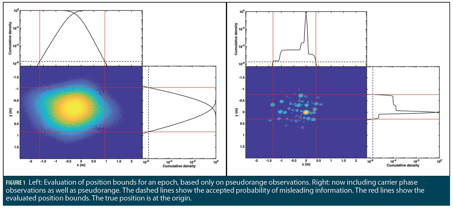
There is however an alternative approach: rather than explicitly resolving ambiguities, it is possible to form position bounds by integrating over all the possible ambiguity solutions. The PDF of the solution is calculated based on the basic physical states and the position bounds are then obtained by identifying a region of space which encloses the required amount of probability. This is the final ingredient in the overall algorithm, giving very tight bounds.
The added value of our handling of the carrier phase measurements to obtain tight bounds is illustrated in Figure 1. As seen in the figure on the right, integer-ambiguities in the phase data can sometimes generate multiple distinct modes, but the basic approach to forming the position bound will stay the same—the final bounds are selected such that the integrated probability in the bounded area satisfies the requirement.
Now that the backbone of our bounding process has been laid down, it is important to stress two critical points that have a very large impact on the bounding performance:
• selecting measurements that have independent errors (for the errors that are not modeled by a state) to meet the assumptions behind the posterior PDF computation, and
• error model fitting using non-Gaussian distributions, which is critical to provide valid position bounds.
Selecting Suitable Epochs and Measurements
Probably the biggest problem when considering automotive integrity schemes is that the local multipath environment is much less stable and predictable than in the aviation environment. Such situations can lead to particularly bad conditions in which multiple signals are subject to non-line-of-sight (NLOS) propagation, for instance when the vehicle is parked under the canopy in a fueling station. This presents a major problem for integrity.
These signals have error characteristics that are radically different to nominal propagation, and mixing the two populations will generate error models that have very broad tails (and that poorly represent each of the populations individually). Also, the degraded environment case might have multiple signals affected simultaneously. This is a strong source of non-independence in the measurement errors, which is a major problem as practical integrity approaches generally make some kind of assumption about the independence of measurement errors.
Our response is therefore to aim at:
• detecting individual signals that are subject to NLOS or severe multipath effects and remove them from further analysis,
• detecting epochs where we are in a degraded environment affecting a large number of satellites. We treat these epochs as unsuitable for GNSS-only bounding and report no solution, in exactly the same way we would if we had driven into a tunnel and lost all GNSS signals.
The basic mechanism used to check for degraded signals and degraded environments is to look at the delta-phase consistency of data over a short window (a few seconds) around the epoch of interest. The aim here is to look for signals whose phase or pseudorange varies in a way that is inconsistent with the rest of the signals. From a physical perspective, this reveals signals that are coming from an unexpected direction, typical of NLOS situations. The reason why we specifically look at pseudorange and carrier phase variation is for statistical independence in downstream analysis. As described earlier, SEPB is a single epoch method that is insensitive to the delta-phase measurements. This separation helps keep the actual data independent.
Our consistency check extends from previous research looking at robust methods for evaluating changes in position and clock over intervals of time. This original work used the classic RANSAC method to look for sets of consistent signals, and to identify outliers. The method works quite well, but it has some limitations:
• It is a stochastic method and a large number of random samples may be needed to gain confidence in the result;
• It is limited to only looking at two epochs.
We therefore replaced the method with a robust least squares minimization using multiple epochs and non-Gaussian loss functions to allow discovery of the consensus solution even when outliers are present in the data. It is referred to as a window-based (WB) selection mechanism.
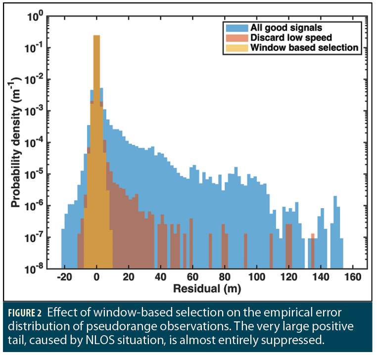
Checking for individual signals that are inconsistent with other signals is a very effective means to discard a small number of measurements that are being affected by some local multipath feature. However, if the environment becomes severely degraded, discarding individual measurements will not be sufficient. Instead, we would prefer to simply mark the whole epoch as being bad, and output that no GNSS measurements are available. This can be done by using simple thresholds on the number of good and bad signals passing the WB selection process.
As a final note, it is important to highlight that this method will only work when the vehicle is moving. When parked, it will not be sensitive to the ray direction, and even NLOS signals will appear consistent. In this situation, none of the signals can really be regarded as being trustworthy and they are thus discarded.
The effect of this WB selection process is quite dramatic, as shown in Figure 2.
At this stage, we can rely on a good method of rejecting almost all outlier measurements. The next step is to form an error model for the remaining high-quality signals.
Fitting Non-Gaussian Error Models
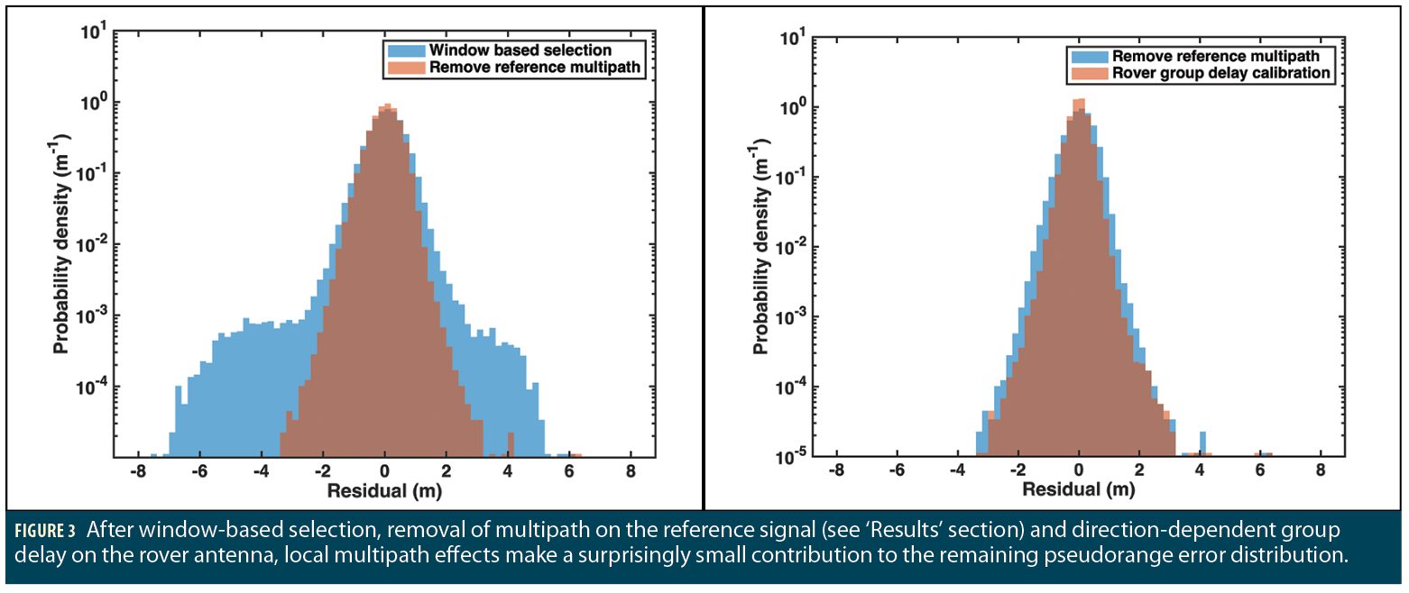
The raw empirical errors on measurements come from a few different sources, and it turns out that some of these error sources can be effectively mitigated, but only if the error sources have been understood in detail. We have therefore taken a forensic approach to our measurement errors, aiming to understand in detail the underlying sources of error, rather than lumping errors from multiple sources into one model. Figure 3 shows the contribution of various sources to the overall error assuming an RTK-like system; the final (irreducible) error due to local multipath effects makes a surprisingly small contribution (remember that measurements during which the user is static are discarded by our selection process).
As can be understood from earlier descriptions, SEPB relies on the use of fitted distributions to represent the true errors. In this sense, the fitting of error model distributions is a critical aspect of the overall system. Any differences between the real error distributions and the fitted models could undermine the overall bound calculation, so it is important to have a good match. This contrasts with traditional approaches, where the aim is to identify measurement error models that provide an overbound on the true error distribution. This is an interesting area of differentiation of SEPB that comes from the fact that SEPB is not based on a linear system.
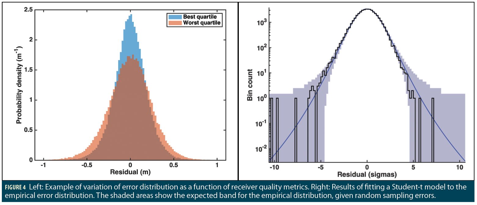
The fitting of the residual data is done via a maximum likelihood approach. For the pseudorange residuals, we pick a Student-t distribution because it provides a good match to the observed distributions (after our measurement selection process), whilst being simple (only one extra free parameter compared to a Gaussian model) and numerically fast to evaluate.
For SEPB to work, the fitting of the residual data has to be conditioned to the current reception conditions for each signal. The fitted model has thus been made dependent on several quality metrics that have been observed to be representative, together, of these reception conditions. An example of the variation of the error distribution is represented in Figure 4 (left) while an example of a fitted distribution, for a given value of the quality indicators, is shown in Figure 4 (right).

Results
u-blox has developed a measurement system that enables collection of large volumes of road driving data and (more importantly) to analyze and characterize the measurement errors with very high accuracy across two bands and all four major GNSS constellations.
The system under test during road trial data collection uses u-blox receivers with a specific firmware. Multiple antennas on the roof are used to represent different system setups, although only one setup will be shown in the following results. Dual frequency measurements from GPS (L1 C/A, L2C), Galileo (E1, E5b), GLONASS (L1 C/A, L2 C/A) and BeiDou (B1I and B2I) were collected.
In the present case, the positioning system is aided by a network of reference stations. The measurements from these reference stations are carefully corrected for local multipath and antenna group delay and phase center offset. These measurements are then used to generate corrections from a non-physical reference station. The maximum baseline to the closest reference station is typically lower than 20 km, resulting in very small residual atmospheric error after correction. Finally, a careful calibration of the user antenna group delay variation was performed and used to further correct the measurements. At the end, the measurement errors are dominated by local errors such as multipath and thermal noise as already presented in Figure 3.
A most fundamental step is the calculation of truth data. This is done using a very expensive and high-quality truthing system, comprised of a high-end reference antenna and receiver and high-quality IMU and wheel tick sensors together with an in-house-developed RTK system using a network of reference receivers to provide local correction signals.
The combination with high-quality inertial measurements and the use of batch calculations over several hours of data allows us to obtain RTK solutions (with integer phase ambiguities resolved), thus allowing true position states to be determined with sub-cm accuracy. At the same time, it is possible to extract true values for the large number of nuisance states that affect the solution. Thanks to the error extraction, it is then possible to perform the error fitting key to SEPB.
This RTK solution is very carefully validated, as problems at this stage could cause serious difficulties during both error modelling and performance evaluation for the overall integrity system. As understood from earlier descriptions, SEPB bound computation is based on:
• the computation of the posterior state PDF assuming fitted (non-Gaussian) error models, and
• a numerical integration of this posterior PDF using a form of MCMC sampling.
The outcome of the bound computation directly provides a lower and an upper position bound on the position. The position estimate is assumed to be the center of this interval.
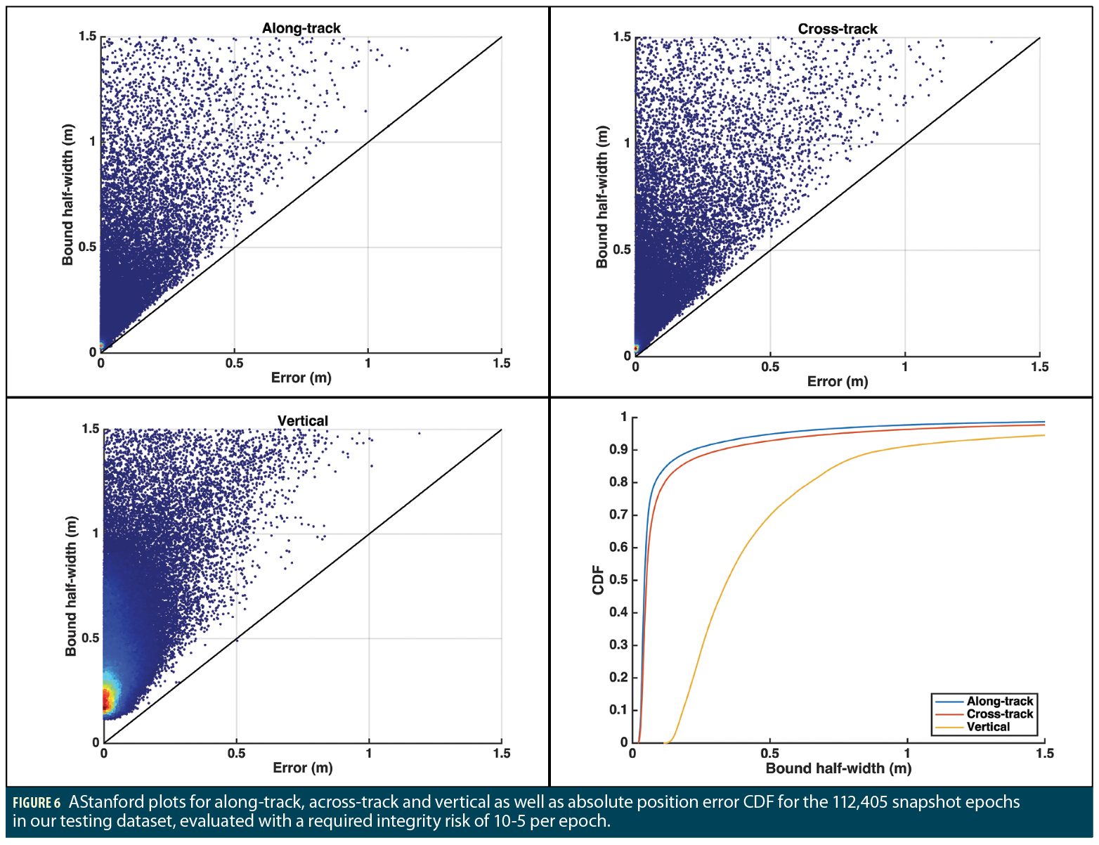
The SEPB mechanism provides a very nice framework for validation. Because it relies on fitted distributions that are conditioned to represent the reception conditions, the targeted percentile associated to the bound computation should be directly observable when enough data is tested. For instance, if the targeted percentile is 10-5 per epoch, then the position error should exceed the SEPB bound roughly once per 100,000 epochs. With this in mind, we have used a subset of all scenarios that provided us with 112,405 epochs during which SEPB could be computed (that means after discarding epochs rejected by the WB selection process) and set the targeted percentile for the bound to 10-5 per epoch. The environment encountered in these scenarios is typical of road environments, with sections in open and in urban areas. The results are shown in Figure 5 for the along, across, and vertical axis.
Some interesting observations:
• The magnitudes of the bounds are small, typically at the decimeter level for the along and across tracks. This shows the impact of the use of carrier-phase measurements in SEPB. Of course, this corresponds to a targeted bound percentile of ‘only’ 10-5 per epoch, but early results with a much lower percentile (10– 5 per hour) have shown that the bounds would remain largely below 1 meter.
• Second, the Stanford plots show that the upper left part of the first diagonal is filled in a fairly uniform way compared to typical Stanford plots in which the points are mostly ‘vertical’ in the left part of the graph. The reason for this is that SEPB relies on dynamic fitted distribution, rather than on Gaussian overbounds. As a consequence, the bounds are more directly linked to the true error.
• Finally, only 1 SEPB bound on a given axis (vertical) is below the actual position error. This is in line with the choice of the targeted percentile and the amount of data. This shows that the implementation of SEPB, and particularly the fitting process and the numerical integration, are appropriate.
Conclusion and Way Forward
A new mechanism to compute position bounds relies on:
• a strict measurement and epoch selection mechanism that ensures that selected measurements are not significantly corrupted by NLOS situations,
• a Bayesian estimation process that allows use of non-Gaussian error models,
• an error fitting model that accounts for quality indicators representative of the reception conditions, and
• an advanced numerical integration to efficiently compute the position bounds.
This mechanism could take great advantage of the carrier phase ambiguities which, combined with the adaptive fitted error models, resulted in along and across track protection level in the decimeter range most of the time in a typical road environment. Moreover, this is done in a rigorous mathematical framework that could facilitate testing and certification. This is a significant achievement compared to existing methods proposed for terrestrial users.
Of course, further work is required to bring this bounding mechanism in an overall integrity concept fitting with automotive applications requiring safe positioning. This includes for instance the use of PPP or PPP-RTK corrections or the management of rare GNSS failures. These aspects and others are being worked upon actively.
Authors

Olivier Julien is a senior principal engineer at u-Blox. His primary activities are related to GNSS receiver signal processing and reliable navigation for critical applications. He received his Ph.D. from the University of Calgary, Canada.

Rod Bryant is Senior Director, Technology at u-blox and leads research and development in all areas of GNSS for positioning and timing. He received his Ph.D. from University of Adelaide, Australia.

Chris Hide is a senior principal engineer at u-blox. His work focusses mainly on high precision GNSS positioning and integrity. He received his PhD from the University of Nottingham, UK.

Ian Sheret is an independent technical consultant specializing in algorithm design for data fusion and inference. He is a founder and director at consulting firm Polymath Insight Limited, and received a Ph.D. in Astrophysics from the University of Edinburgh.


