
A new perspective on positioning safety analyses.
SEBASTIAN CIUBAN, PETER J.G. TEUNISSEN, CHRISTIAN C.J.M. TIBERIUS, DELFT UNIVERSITY OF TECHNOLOGY
Positioning via Global Navigation Satellite Systems (GNSS) and Terrestrial Networked Positioning Systems (TNPS), along with measurements from other sensors (e.g., inertial measurement units, cameras, LiDAR), is widely used or of growing interest in several safety-critical applications, such as automotive, aviation, rail and maritime [1-3]. With these measurements, or observables, a position estimator x̅∈Rn can be formulated, where n≥1 represents the dimension (e.g., n=1 for vertical component, n=2 for horizontal components). Given access to the probability density function (PDF) of x̅∈Rn, denoted fx̅(x), and an application specific safety-region B⊂Rn (e.g., interval when n=1, ellipse when n=2), one can pose the following question: “What is the probability that the position estimator falls outside the designated safety-region?”
Quantifying this probability enables its comparison against application-specific requirements, or guidelines, to determine whether they are satisfied. This probability can be viewed as a positioning “safety indicator” for the application of interest.
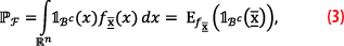
We formulate the aforementioned probability based on the event of positioning failure F=(x̅∉B) [4], and express it as follows
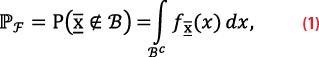
where Bc=Rn\B is the complement of the safety-region (i.e., the Rn space without the safety-region B). The computation of PF is a challenging task, primarily because the PDF fx̅(x) may have multiple modes. These modes arise from the position estimator, which, as we assume here, usually results from a combined parameter estimation and statistical hypothesis testing procedure to accommodate for model misspecifications (e.g., faults or outliers in observables). This intricacy is captured in the theoretical framework introduced in [5].
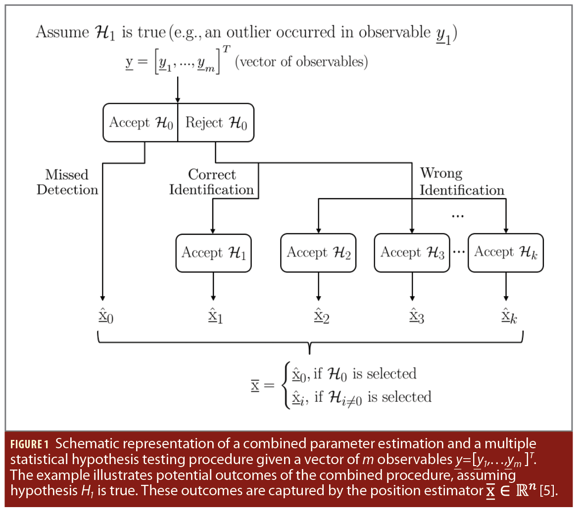
To account for such model misspecifications, one can assume a positioning model that is valid under nominal conditions (the null hypothesis H0) and design alternative positioning models under multiple alternative hypotheses Hi≠0 with i∈{1,…,k}. For example, in the case of GNSS-based positioning, one can define positioning models under the Hi≠0’s to account for the presence of one or multiple outliers (or faults) in the code-based observables, cycle slips in the phase-based observables, satellite failures, unmodelled atmospheric delays, etc. Then the objective is to select the most likely hypothesis and use the corresponding positioning model to provide the position estimator x̅i for i∈{0,…,k} (Figure 1). As shown in Figure 1, we highlight that the position estimator x̅∈Rn is a function of the individual estimators x̅i and the statistical testing procedure used to select these estimators (e.g., a Detection Identification and Adaptation-DIA procedure [6-8] or a Fault Detection and Exclusion-FDE procedure [9-11]).
The expression of fx̅(x) provides additional insights into its dependencies [5]
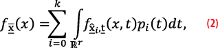
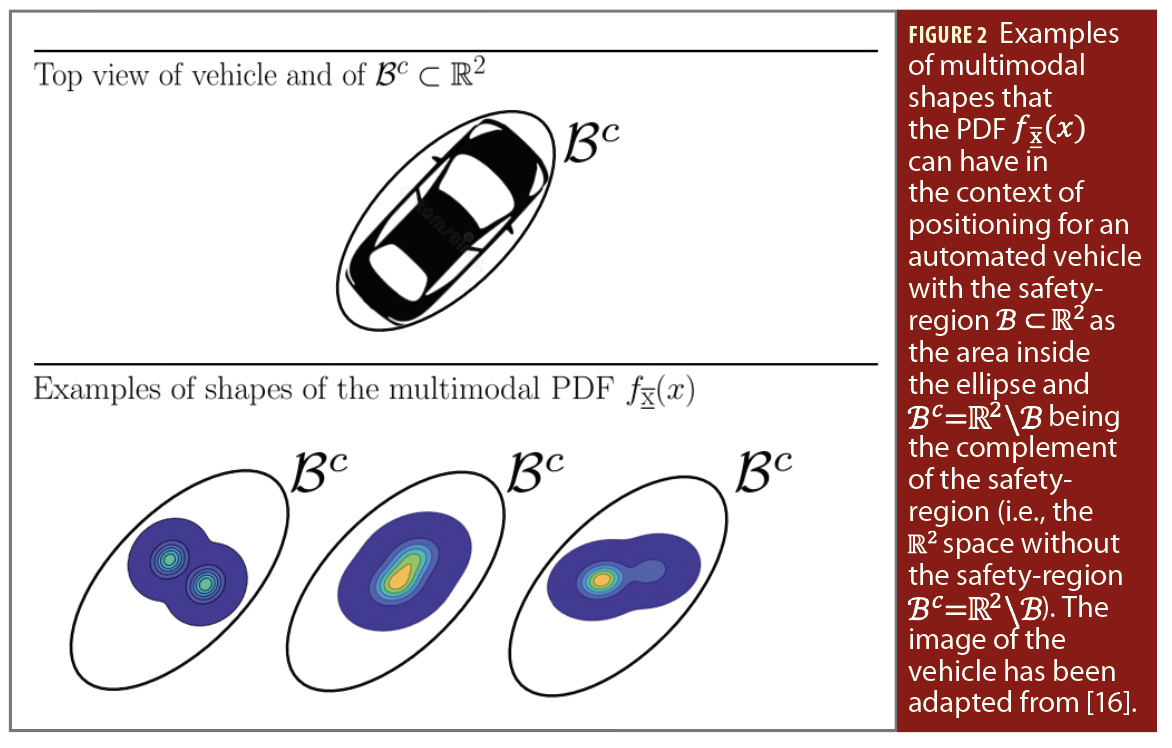
where fx̅i,t̅(x,t) is the joint PDF of the individual estimators x̅i∈Rn and the vector of misclosures t̅∈Rr used to construct statistical tests for selecting the most likely hypothesis Hi, and pi(t̅) is an indicator function that equals 1 if Hi is selected and 0 otherwise. The vector of misclosures has the dimension of the measurement redundancy, denoted r, and it contains all the available information useful for testing the validity of the positioning model under H0. From the expression of fx̅(x) in (2) we emphasize that PF from (1) depends on the number of k+1 hypotheses, on the dimension n of the to-be-estimated parameter vector, and also on the dimension r of the misclosure vector. Furthermore, x̅i∈Rn and t̅∈Rr are dependent for i≠0, which means the joint PDF cannot be expressed as a product of the marginal PDFs (i.e., fx̅i,t̅(x,t) ≠ fx̅i(x) ft̅(t̅), for i≠0). Ignoring or failing to account for the dependence between x̅i∈Rn and t̅∈Rr, for i≠0, may result in overly-optimistic results when computing PF, potentially leading to incorrect conclusions that positioning safety requirements are met when they are not [12-15]. The multimodal structure of fx̅(x) (Figure 2) and its aforementioned dependencies render analytical methods for computing PF unfeasible.
Another aspect to take into account when computing PF is related to the requirement for the event of positioning failure F=(x̅∉B)= (x̅∈Bc) to be rare (e.g., PF<10-7 [17]). Because analytical methods for computing PF are unfeasible, numerical integration methods are reasonable candidates. However, as the rarity requirement for F=(x̅∈Bc) becomes more stringent, the computational effort required to compute such probabilities increases significantly. In recent work, we tackled these challenges by introducing a method grounded in rare event simulation principles and proposed a possible approach to address them [18]. The method is intended for use during the design stage of positioning algorithms, where decisions are required regarding (i) measurement models associated with selected positioning technologies and sensors, (ii) parameter estimation techniques for the position vector, (iii) statistical hypothesis testing procedures to accommodate for model misspecifications, and (iv) positioning scenarios of interest (e.g., vehicle driving on a highway, or in an urban area), among other considerations. This methodology is consistent with the scenario-based safety assessment framework widely adopted for studies on automated and autonomous vehicles [19-21].
In this contribution, we outline the principles underlying the approach proposed in our recent work [18]. As an example, we present a simulation-based analysis of positioning safety for an automated vehicle using a real dual-constellation GPS and Galileo satellite geometry [13].
Standard Monte Carlo and Importance Sampling
A reasonable first step is to use numerical integration methods, such as standard Monte Carlo (MC) simulation, to compute PF. It is possible to re-express (1) as an expected value with respect to the PDF fx̅(x), denoted Efx̅(.),
where 1Bc(x̅) is an indicator function that is 1 if x̅∈Bc, and 0 otherwise. By generating Nx̅ independent and identically distributed (i.i.d.) pseudo-random samples from fx̅(x) one can approximate (3) as follows (based on counting how many pseudo-random samples fall in Bc=Rn\B)
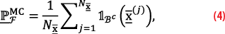
with its simulation variance, or dispersion, expressed as D(P̅FMC)= PF(1-PF)/Nx̅. However, the standard Monte Carlo approximation in (4) has limitations when computing probabilities of rare events. Specifically, in the case of rare events a substantial number of pseudo-random samples Nx̅ is needed to be able to compute (4) with a low simulation variance D(P̅FMC). For example, if the objective is to compute a target value PF=10-9 with √(D(P̅FMC))=10-10, then the required number of pseudo-random samples would be Nx̅≈1011, which involves an excessively large computational effort.
To tackle the limitations of the standard Monte Carlo method, a different approach is needed. Importance Sampling (IS) is a reasonable candidate to be considered as it can achieve simulation variance reduction without a significant increase of the required pseudo-random samples to be generated [22]. The principles of IS have found applicability across a wide area of safety-critical applications, such as safety analyses of structures, nuclear power plants, and for computations of probabilities of collision events in aviation [23-25]. On the basis of IS, we can express PF from (3), with respect to a newly introduced PDF f̃(x), as follows
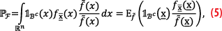
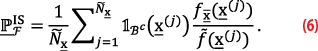
where f̃(x) is also called IS density, auxiliar density, or proposal PDF [23, 26]. The main idea is to choose, or find, a proposal PDF that has a larger probability density over the region Bc=Rn\B than fx̅(x) and 1Bc(x̅) f̃(x)≠0 whenever 1Bc(x̅) fx̅(x)≠0 [27]. If such proposal PDF f̃(x) is chosen, then by generating Ñx i.i.d. pseudo-random samples from it allows for the approximation of (5) as follows
The performance of P̅FIS in reducing simulation variance depends on the choice of the proposal PDF f̃(x), which in turn drives the quality of the probability estimates. It is possible to find a proposal PDF f̃(x), within a family of PDFs (e.g., exponential family) that minimizes the Kullback-Leibler (KL) divergence, or equivalently the Cross-Entropy, with respect to the optimal theoretical PDF f̃*(x)=[1Bc(x̅) fx̅(x)]/PF [22]. The theoretical PDF f̃*(x) is optimal in the sense that it minimizes simulation variance. In practice, f̃*(x) cannot be used because it depends on the unknown PF. The proposal PDF f̃(x) that minimizes the KL divergence w.r.t. f̃*(x) can be determined using the Cross-Entropy method [28].
Probability of Positioning Failure and its Components
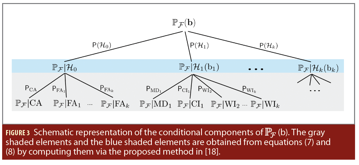
We recently proposed a method [18] that can compute the probability of positioning failure from its conditional components (Figure 3). A component-wise computation of PF enables the determination of the conditional components that contribute most, or least, to its value. Having designed a statistical hypothesis testing procedure to address model misspecifications with a null hypothesis H0 (comprising of the positioning model believed to be valid under nominal conditions) and k alternative hypotheses Hi≠0 (e.g., comprising of positioning models that account for the presence of outliers, or faults, in the observables), it is possible to decompose PF into its conditional components based on the statistical testing decisions: Correct Acceptance (CA) when H0 is accepted and H0 is valid; False Alarm (FAi) when Hi≠0 is accepted and H0 is valid; Missed Detection (MDi) when H0 is accepted and Hi≠0 is valid; Correct Identification (CIi) when Hi≠0 is accepted and Hi≠0 is valid; Wrong Identification (WIj) when Hj is accepted and Hi is valid for j∉{0,i} (see also the example in Figure 1). This decomposition has been presented and elaborated on in [13]. A graphical representation of the “failure-tree” is shown in Figure 3, where the notation of the probability of positioning failure changed to PF(b̅) with b̅={b̅1,…,b̅k} to account for b̅i, with i∈{1,…,k}, under all the k alternative hypotheses. Note: Figure 3 goes here The equations that describe the branches and connections in Figure 3 are the following:
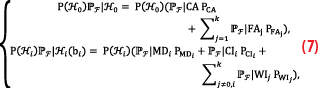
where P(H0) and P(Hi), for i∈{1,…,k}, are the apriori probabilities of the hypotheses H0 and Hi≠0, PF|E is the probability of positioning failure conditioned on the statistical testing decision E∈{CA,FAi,MDi,CIi,WIj}, and PE is the probability of the event of the statistical decision E. Once the conditional components from (7) are computed, then the total probability of positioning failure is obtained as follows [18],

With (7) and (8) one can obtain the entire characteristic of PF(b̅) as a function of b̅={b̅1,…,b̅k}, thus providing all the information required to perform a rigorous sensitivity analysis for the design purposes of the positioning system. The positioning safety-analysis in the next section is based on constructing the “failure-tree” in Figure 3 via the computations of (7) and (8). Because the size of the outliers in (8) is not known a priori, the maximum value of (8) is reported to provide insights into the worst-case scenario, aiding in the assessment of whether safety requirements or guidelines are met.
Decimeter Level GNSS-Based Positioning Safety Analysis
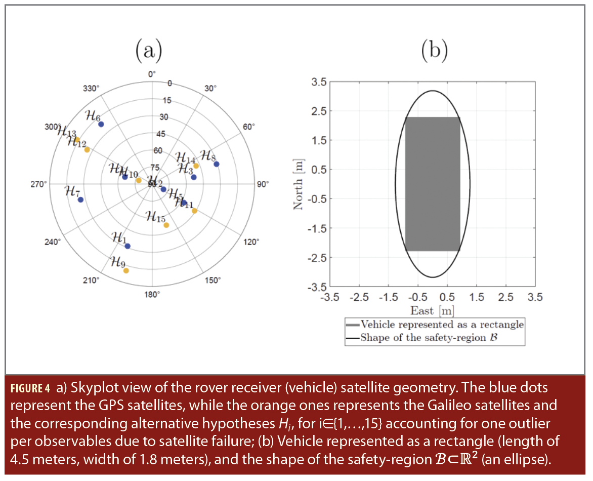
We consider the GNSS-based positioning safety analysis presented in [13], which is also similar to the one in [18]. The simulation scenario involving an automated vehicle which coordinates are determined in a local East-North-Up (ENU) coordinate system using single-frequency, code-based pseudorange observables in a Differential (DGNSS) setup. The GNSS constellations we consider are GPS (G) and Galileo (E), at L1/E1 frequency. At the considered snapshot of time (epoch), eight GPS and seven Galileo satellites are visible after applying an elevation mask of 10°. Figure 4(a) shows the skyplot of the observed GPS and Galileo satellites by the automated vehicle. Additionally, an elevation depending weighting is applied to the observables.
The horizontal positioning precision is about 0.5 meters (95% circular probability radius).
In the setup of the statistical hypothesis testing procedure to accomodate for outliers or faults in measurements, in this case the DIA procedure, we account for individual outliers, assuming only one occurs at a time (there are k=15 alternative hypotheses). At the output of this procedure the DIA-estimator x̅∈Rn and its PDF fx̅(x) are obtained. When determining, or choosing, the shape and size of the safety-region B⊂R2 several factors should be considered, such as: (i) vehicle’s dimensions, (ii) road geometry to ensure the vehicle is within its lane, (iii) minimum required braking distance as a function of the vehicle’s speed, (iv) proximity with regard to other traffic participants, among other considerations. Several approaches have been proposed in terms of shapes of the safety-region that bound the vehicle (e.g., elliptical, rectangular) in several studies [17, 29, 30]. For our scenario, and for consistency with existing approaches in the literature, we choose an ellipse to inscribe the vehicle, which has a length of 4.5 meters, a width of 1.8 meters, and an orientation of 0° relative to the North axis (Figure 4(b)).
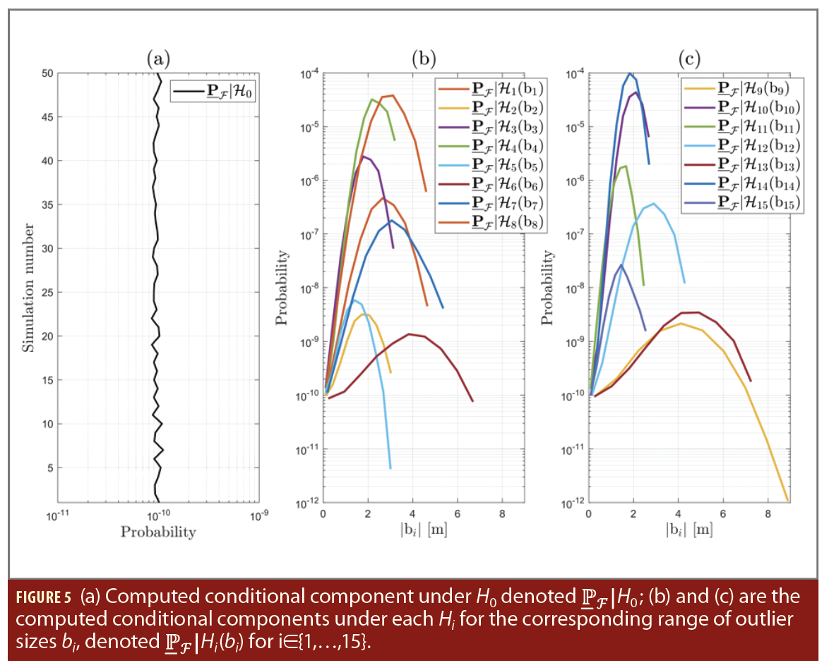
With the DIA-estimator x̅∈Rn, its PDF fx̅(x), and the ellipsoidal safety-region B⊂R2 defined, the method in [18] can be applied for positioning-safety analysis. This yields the computed conditional components of P̅F(b̅) from equation (8). Figure 5(a) shows the component P̅F|H0 computed over 50 simulation runs to observe the variability in the results, and Figures 5(b) and 5(c) show the P̅F|Hi(b̅i) as a function of the outlier size b̅i for i∈{1,…,15}. It is noticable that P̅F|H4(b̅4), P̅F|H8(b̅8), P̅F|H10(b̅10), and P̅F|H14(b̅14) are dominating when the size of their respective outlier is larger than 1.60 meters. This can be explained based on the rover receiver-satellite geometry in Figure 5(a), which shows that satellites corresponding to the hypotheses 4, 8, 10, and 14 have a large influence on the horizontal-axis (east-component) of the 2D position solution. Conversely, satellites at low-elevations have a reduced contribution to the 2D position solution (e.g., 6, 9, and 13), which leads to low probabilities of positioning failure under the respective alternative hypotheses.
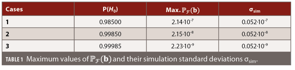
To compute the maximum P̅F(b̅), assumptions are needed for the a-priori P(Hi) for i∈{0,…,15}. Because the alternative hypotheses account for outliers in the pseudoranges at the rover-receiver (automated vehicle), it is assumed they primarily occur due to different signal reflections caused by the surrounding environment (e.g., nearby infrastructure). For this analysis, we consider three sets of assumptions ranging from conservative to optimistic cases: (1) P(H0)=0.98500 and P(Hi)=10-3 for i∈{1,…,15}; (2) P(H0)=0.99850 and P(Hi)=10-4 for i∈{1,…,15}; (3) P(H0)=0.99985 and P(Hi)=10-5 for i∈{1,…,15}. The obtained results for the maximum P̅F(b̅) in the three cases are shown in the Table 1. Note these results correspond to the rover receiver-satellite geometry in Figure 4(a) and the fixed safety-region B⊂R2 in Figure 4(b).
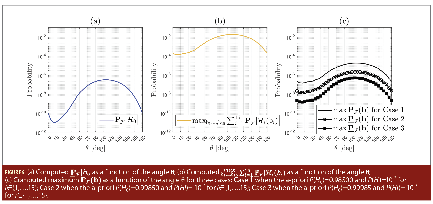
In practice, a vehicle will change its orientation while moving (e.g., when making a U-turn, exiting a highway, taking a left/right turn), and consequently, the maximum P̅F(b̅) will also change. For a short time window (e.g., few minutes), it can be assumed the rover receiver-satellite geometry from Figure 4(a) is constant, allowing us to base our next analysis on the vehicle’s change in the orientation angle θ (measured, in degrees, clockwise with respect to the North axis). Therefore, the safety region Bθ⊂R2 (note the change in notation) will also depend on the vehicle’s orientation angle θ. The objective is to compute the maximum P̅F(b̅) as a function of θ from its components P̅F|H0 and maxb̅1,…,b̅15 ∑i=115 P̅F|Hi(b̅i). Figure 6(a) shows the results of P̅F|H0 as a function of θ and that the maximum values is 3.33⋅10-7±0.0216⋅10-7 for the vehicle’s orientation angle of θ=110°. In the case of the component maxb̅1,…,b̅15 ∑i=115 P̅F|Hi(b̅i), as shown in Figure 6(b), the maximum value is reached at 1.81⋅10-2 ±0.00462⋅10-2 for θ=110°. By combining the results from Figure 6(a) and Figure 6(b) with the assumptions regarding the a-priori probabilities P(H0) and P(Hi) for i∈{1,…,15} as discussed in the three cases, the results in Figure 6(c) are obtained. Note: Figures 6a, b and c go here In the most conservative case (Case 1), the maximum P̅F(b̅) at θ=110° is 1.84⋅10-5 ±0.000216⋅10-5 while for the most optimistic case (Case 3) the maximum P̅F(b̅) is 4.94⋅10-7 ±0.0216⋅10-7. These results help determine whether the target requirements or guidelines for positioning safety are met. If the requirements or guidelines are not satisfied, it may be necessary to make appropriate changes to the positioning algorithm design choices. These could include aspects such as the measurement setup (e.g., functional and stochastic models), the safety-region, or the combined parameter estimation and statistical hypothesis testing procedure. For instance, the new theoretical framework introduced in [31] shows how fit-for-purpose statistical hypothesis testing improves the performance of DIA-estimators.
Summary and Conclusions
In this contribution, we have presented a new perspective on positioning safety analyses by addressing key ideas and challenges associated with the computation of the probability of positioning failure, such as: (i) the multimodal PDF of the position estimator fx̅(x), which accounts for the dependence between parameter estimation and statistical hypothesis testing to accommodate potential faults or outliers in the measurement model; (ii) to account for the dependencies on the number of k+1 hypotheses, on the dimension n of the to-be-estimated parameter vector, and also on the dimension r of the misclosure vector when constructing the PDF fx̅(x) and performing its integration over the region Bc= Rn\B (the Rn space without the safety-region B⊂Rn), which renders analytical methods overly complex or impractical; and (iii) the rarity of positioning failure events in the context of safety-critical applications, which requires more advanced numerical integration methods than standard Monte Carlo.
To address these challenges, we presented an approach based on our recent work in [18], which relies on techniques from rare event simulation, specifically Importance Sampling and the Cross-Entropy Method [22, 28]. The computation and analysis of the probability of positioning failure are intended to be performed during the design stage of positioning algorithms, where key decisions are made regarding (i) measurement models, (ii) parameter estimation methods for the position vector, (iii) statistical hypothesis testing procedures to handle model misspecifications (e.g., outliers or faults in measurements), and (iv) positioning scenarios for vehicles, among other factors. This approach aligns with scenario-based safety assessment frameworks, which are widely used or proposed in studies on automated and autonomous vehicles [19-21].
As an example, we applied the proposed method to perform a single-epoch positioning safety analysis for an automated vehicle, focusing on decimeter-level precision GNSS-based positioning. The method facilitated an analysis of a worst-case scenario aimed at determining the maximum probability of positioning failure. Such analyses can guide decisions on whether positioning safety targets or requirements are satisfied. Once compliance with application-specific requirements is demonstrated based on the probability of positioning failure in the relevant scenarios, the corresponding parameter estimation and statistical hypothesis testing procedure can be implemented for real-time positioning.
While the chosen positioning scenario was centered on the automotive domain, the proposed approach for computing and analyzing the probability of positioning failure is also applicable to other safety-critical fields, including civil aviation, shipping and rail.
Acknowledgements
This research was funded by the Dutch Research Council (NWO) under Grant 18305, titled ‘I-GNSS Positioning for Assisted and Automated Driving.’ The support is gratefully acknowledged.
References
(1) P. J. G. Teunissen and O. Montenbruck, Eds., Handbook of Global Navigation Satellite Systems. Springer, 2017.
(2) Y. T. J. Morton, F. van Diggelen, J. J. Spilker Jr., B. W. Parkinson, S. Lo, and G. Gao, Eds., Position, Navigation, and Timing Technologies in the 21st Century: Integrated Satellite Navigation, Sensor Systems, and Civil Applications. Wiley, IEEE Press, 2020.
(3) J. C. J. Koelemeij, et al., “A hybrid optical-wireless network for decimetre-level terrestrial positioning,” Nature, vol. 611, no. 7936, pp. 473-478, Nov. 2022.
(4) RTCA-Special Committee 159, “Minimum Operational Performance Standards (MOPS) for Global Positioning System/Satellite-Based Augmentation System Airborne Equipment,” DO-229F, Radio Technical Commission for Aeronautics, pp. 15, 2020.
(5) P. J. G. Teunissen, “Distributional theory for the DIA method,” Journal of Geodesy, vol. 92, no. 1, pp.59-80, 2018.
(6) W. Baarda, “A Testing Procedure for Use in Geodetic Networks,” Netherlands Geodetic Commission, Publications on Geodesy, 2(5):1–97, 1968.
(7) I. Gillissen and I. A. Elema, “Test results of DIA: A real-time adaptive integrity monitoring procedure, used in an integrated navigation system,“ International Hydrographic Review, vol. 73, nb. 1, pp.75-103, 1996.
(8) P. J. G. Teunissen, “Batch and Recursive Model Validation,” Chapter 24 in Springer Handbook of Global Navigation Satellite Systems, P. J. G. Teunissen and O. Montenbruck, Eds., Springer, pp. 687-720, 2017.
(9) P. T. Hwang and R.G. Brown, “RAIM-FDE Revisited: A New Breakthrough in Availability Performance With nioRAIM (Novel Integrity-Optimized RAIM),” NAVIGATION, 53(1):41–51, 2006.
(10) L. Yang, Y. Li, and C. Rizos, “An enhanced MEMS-INS/GNSS integrated system with fault detection and exclusion capability for land vehicle navigation in urban areas,” GPS Solutions, vol. 18, no. 4, pp.593-603, 2013.
(11) J. Blanch et al., “Baseline Advanced RAIM User Algorithm and Possible Improvements,” IEEE Aerospace and Electronic Systems, 51(1):713–732, 2015.
(12) S. Ciuban, P. J. G. Teunissen, and C. C. J. M. Tiberius, “Dependence Between Parameter Estimation and Statistical Hypothesis Testing: Positioning Safety Analysis for Automated/Autonomous Vehicles,” IEEE Transactions on Intelligent Transporation Systems, vol. 26, no.4, pp. 5509 – 5521, 2025.
(13) S. Ciuban, P. J. G. Teunissen, and C. C. J. M. Tiberius, “GNSS Positioning Safety: Probability of Positioning Failure and its Components,” Proceedings of the 37th International Technical Meeting of the Satellite Division of the Institute of Navigation (ION GNSS+), pp. 2228-2249, 2024.
(14) S. Zaminpardaz and P. J. G. Teunissen, “On the computation of confidence regions and error ellipses: A critical appraisal,” Journal of Geodesy, vol. 96, no. 10, pp.1-18, 2022.
(15) S. Zaminpardaz, P. J. G. Teunissen, and C. C. J. M. Tiberius, “Risking to underestimate the integrity risk,” GPS Solutions, 23(29):1–16, 2019.
(16) Wikimedia Commons, Citroen C3, top. Available: https://commons.wikimedia.org/wiki/File:C3top.png#file.
(17) Reid, T. G. R. et al., “Localization Requirements for Autonomous Vehicles,” in SAE International Journal of Connected and Automated Vehicles, 2019.
(18) S. Ciuban, P. J. G. Teunissen, and C. C. J. M. Tiberius, “A Method to Compute the Probability of Positioning Failure for Vehicles in the Context of Dependence Between Parameter Estimation and Statistical Hypothesis Testing,” IEEE Transactions on Vehicular Technologies, vol. 74, no.10, pp. 15238 – 15253, 2025.
(19) S. Riedmaier et al., “Survey on Scenario-Based Safety Assessment of Automated Vehicles,” IEEE Access, vol. 8, pp.87456-87477, 2020.
(20) U.N.E.C.E., “New Assessment/Test Method for Automated Driving (NATM) Guidelines for Validating Automated Driving Systems (ADS),” United Nations Economic Commission for Europe–Inland Transport Committee, Report, 2023.
(21) E. de Gelder et al., “TNO Street Wise: Scenario-Based Safety Assessment of Automated Driving Systems,” Netherlands Organisation for Applied Scientific Research (TNO), White Paper, 2024.
(22) H. Kahn and A. W. Marshall, “Methods of Reducing Sample Size in Monte Carlo Computations,” Journal of the Operations Research Society of America, vol. 1, no. 5, pp.263-278, 1953.
(23) I. Papaioannou, C. Papadimitriou, and D. Straub, “Sequential Importance Sampling for Structural Reliability Analysis,” Structural Safety, vol. 62, pp.~66–75, 2016.
(24) B. J. Garrick, et al., Reliability analysis of nuclear power plant protective systems (Research and Development Report). Holmes and Narver Inc. Nuclear Division, 1967.
(25) M. Mitici and H. A. P. Blom, “Mathematical Models for Air Traffic Conflict and Collision Probability Estimation,” IEEE Transaction on Intelligent Transporation Systems, vol. 20, no. 3, pp.1052-1068, 2019.
(26) R. V. Rubinstein and D. P. Kroese, Simulation and the Monte Carlo Method. Wiley Series in Probability and Statistics, 2008.
(27) G. Biondini, “An introduction to rare event simulation and importance sampling,” Chapter 2 in Handbook of Statistics, V. Govindaraju, V. V. Raghavan, and C. R. Rao, Eds., Elsevier B.V., pp. 29-68, 2015.
(28) R. V. Rubinstein and D. P. Kroese, The Cross-Entropy Method: A Unified Approach to Combinatorial Optimization, Monte-Carlo Simulation, and Machine Learning. Springer Series in Information Science and Statistics, 2004.
(29) Y. Feng, C. Wang, and C. Karl, “Determination of Required Positioning Integrity Parameters for Design of Vehicle Safety Applications,” ION GNSS+, pp. 129-141, 2018.
(30) O. N. Kigotho and J. H. Rife, “Comparison of Rectangular and Elliptical Alert Limits for Lane-Keeping Applications,” ION GNSS+, pp. 93-104, 2021.
(31) P. J. G. Teunissen, “On the Optimality of DIA-Estimators: Theory and Applications,” Journal of Geodesy, vol. 98, no. 43, pp.1-26, 2024.
Authors
Sebastian Ciuban received the M.Sc. in Aerospace Systems: Navigation and Telecommunications from École Nationale de l’Aviation Civile (ÉNAC), Toulouse, France, in 2017. Post-graduation, he joined the European Space Research and Technology Centre (ESTEC) as a Young Graduate Trainee (YGT) in the Directorate of Navigation. From 2019 to 2021, he worked as a GNSS Engineer at CGI Nederland B.V. In 2021, he started a Ph.D at Delft University of Technology, Delft, The Netherlands, in the field of PNT safety for automated and autonomous vehicles (to be defended in December 2025). As of June 2025, he joined the Defense and Security Unit of Science and Technology (S[&]T) B.V, Delft, The Netherlands.
Peter J.G. Teunissen is Professor of Geodesy and Satellite Navigation at Delft University of Technology, the Netherlands, and a member of the Royal Netherlands Academy of Arts and Sciences. His past academic positions include Head of the Delft Earth Observation Institute, Science Director of the Australian Centre for Spatial Information, and Federation Fellow of the Australian Research Council. He has been research-active in various fields of Earth Observation, with current research focused on the development of theory, models and algorithms for high-accuracy applications of satellite navigation and remote sensing systems.
Christian C.J.M. Tiberius received a Ph.D. on recursive data processing for kinematic GPS surveying from Delft University of Technology, Delft, The Netherlands. He is an Associate Professor at the Geoscience and Remote Sensing (GRS) Department, Delft University of Technology. His research interests include navigation with GNSS and terrestrial radio positioning, primarily for automotive applications.