
GBAS corrections are typically only used for precision approaches of large aircraft. This study tests using GBAS corrections and integrity parameters for UAVs.
SOPHIE JOCHEMS, VALENTIN FISCHER, MICHAEL FELUX, ZURICH UNIVERSITY OF APPLIED SCIENCES, CENTER FOR AVIATION
MICHAEL JÄGER, LUCIANO SARPERI, ZURICH UNIVERSITY OF APPLIED SCIENCES, INSTITUTE OF SIGNAL PROCESSING AND WIRELESS COMMUNICATIONS
NATALI CACCIOPPOLI, EUROCONTROL
The Ground Based Augmentation System (GBAS) is a precision approach and landing system that provides corrections for Global Positioning System (GPS) navigation signals to airborne users. Besides corrections, GBAS also provides integrity parameters, allowing users to bound their residual position errors after applying the corrections to the pseudorange measurements of the airborne user equipment. The GBAS station also provides reference coordinates defining the reference approach trajectory guiding aircraft horizontally and vertically toward the runway. All data are broadcast from the ground station via a VHF Data Broadcast (VDB) in a standardized format, as specified in document DO-246E [1]. The broadcast is freely accessible and can be received and decoded by virtually everyone. A GBAS ground station is located within the security perimeter of an airport and uses high-quality antenna and receiver equipment to keep errors introduced by the ground facility to a minimum. Furthermore, it provides guaranteed levels of performance according to specification and continuously self-monitors the integrity of the information provided [2].
This augmentation system in its current operational form only provides a so-called approach service that, by design, serves a very specific purpose. In civil aviation, aircraft equipped with appropriate avionics can use the provided information to correct GPS signals, ensure all integrity requirements are met, and use the information regarding the approach geometry in the GBAS message to fly precision approaches. However, GBAS is not widely used because not many airports are equipped with a GBAS ground station, and depending on the airport, only limited parts of the fleet operating in and out are equipped with the GBAS Landing System (GLS). The reason for this is a classic chicken/egg problem. On the one hand, the Air Navigation Service Provider (ANSP), or in some cases also the airport operator, is responsible for the installation, operation and maintenance of a GBAS ground station. As this is rather expensive, not many ANSPs and/or airports are willing to install such a ground station without a solid business case. Because only a small percentage of aircraft operating at a particular airport are typically equipped to fly a GLS approach, it is difficult to generate operational benefits from a GBAS. On the other hand, it is often not worthwhile for aircraft operators to equip their aircraft with the required receiver, as there are few destinations in their route network where a GLS approach is possible and could bring operational benefits.
Previous works [3,4] explored the possibility of using GBAS-like Local Area Differential GNSS (LADGNSS) for UAV navigation. LADGNSS is similar to GBAS but removes some expensive hardware, making it more suitable to support UAVs while still providing high levels of integrity. As identified in [3,4] and followed up by [5], airborne multipath errors play a critical role for integrity. However, in flight trials with UAVs, residual airborne multipath errors are assumed to be well bounded by the error models developed for large transport aircraft [6,7]. Another paper [8] analyzed the theoretical performance of the envisioned Differentially Corrected Positioning Service (DCPS) for GBAS, a service that enables use-cases other than precision approach guidance of large aircraft by relying on data received from an operational GBAS. For this purpose, GBAS messages transmitted by the ground station at Zurich Airport (ZRH) were received and decoded. The theoretical protection levels at different distances from the ground station for the GBAS DCPS (that differ from the protection levels of the approach service provided by the station but uses the same integrity parameters for error bounding) were then calculated and compared to SBAS protection levels.
The results suggested GBAS could provide operational benefits when staying within a radius of about 57 km from the airport. At distances more than 57 km from the airport, however, GBAS protection levels become larger than SBAS protection levels due to ionospheric and ephemeris error decorrelation and therefore no longer provide any advantage over SBAS.
In this study, we continue our previous work and focus on the use of GBAS corrections in the emerging field of UAV navigation and the potential to operate drones at distances below 50 km from the GBAS ground station. One main challenge when using broadcast corrections is the limited possibitly to receive the VHF-based transmission at the low flight altitudes typical for UAV operations. We explore receiving and decoding GBAS messages near the airport and then applying the corrections and using the integrity parameters for correcting and bounding the positioning errors at the UAV. To this end, we evaluate the performance of the proposed navigation method and discuss operational aspects of GNSS navigation for UAV operations.
Methods
To evaluate navigation performance under realistic conditions, we conducted a flight test using a UAV. In subsequent postprocessing, the flight test data was augmented with recorded corrections and integrity parameters from the GBAS at Zurich Airport.
Data Collection
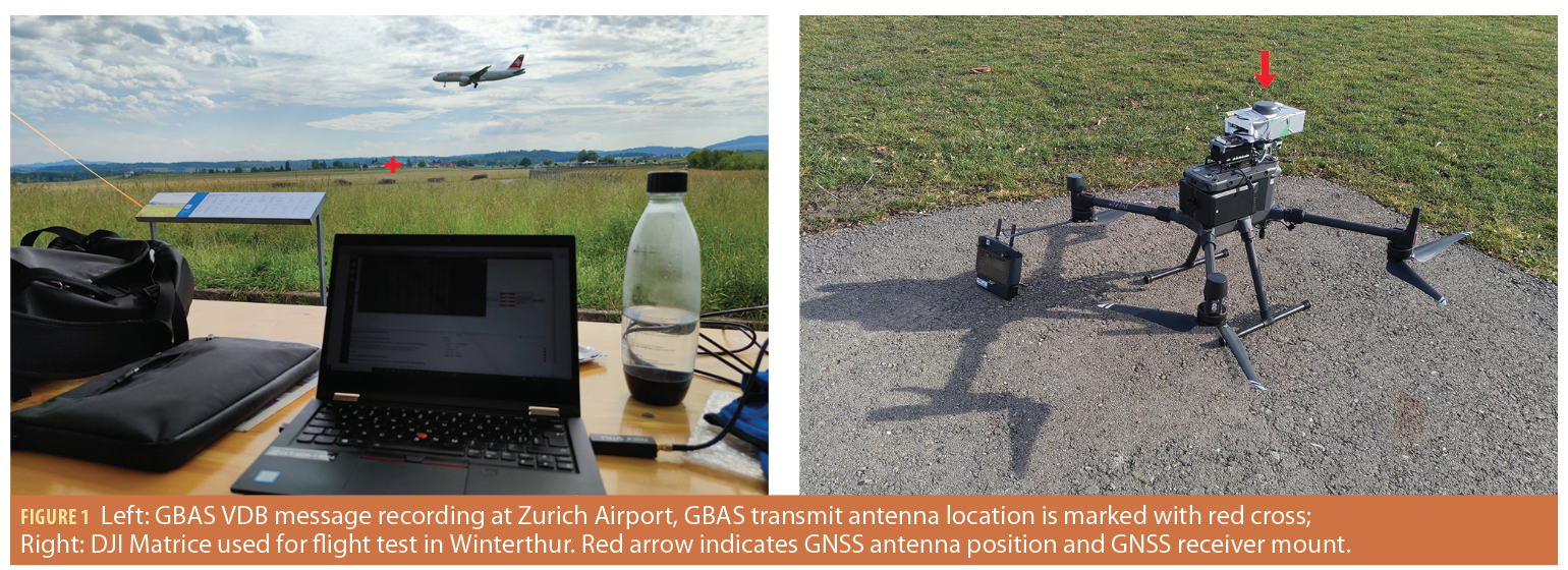
To obtain GBAS corrections, a software-defined radio receiver was set up near Zurich Airport, equipped with a GBAS Approach Service Type (GAST) C ground station. The selected location was within line-of-sight of the VDB transmit antenna, ensuring good signal reception (Figure 1, left). The GBAS was in regular operation at the time of recording, provided corrections and integrity parameters for the approach service, and supported CAT-I operations down to 200 feet above ground to runway 14, which is Zurich Airport’s main landing runway. While a fully operational UAV navigation concept would require near real-time decoding and forwarding of GBAS data via the cell phone network (or a different real-time capable datalink), for this initial study we recorded the GBAS data for later postprocessing together with the GNSS data from the UAV.
The UAV was flown at the glider airfield in Winterthur (ICAO Airport Code LSPH), located approximately 15 km north-east from Zurich Airport, on February 21. A Septentrio mosaic-X5 receiver with a GNSS antenna was mounted on the drone and attached rigidly to the airframe by means of a 3D-printed case. The receiver recorded GPS pseudorange and carrier phase information on L1 and L5, as well as SBAS information. As GBAS and SBAS both only provide corrections and integrity parameters for GPS L1, this information was only used for the performance evaluations conducted in this study.
Two different flight tests and their results are covered in this article. The first test flight carried out in June 2022 contained periods of static hovering at altitudes of 2 m and 5 m above ground to collect GNSS data (pseudorange and carrier phase information) in a stationary scenario but at different altitudes for an initial assessment of the potential impact of ground reflection multipath at different heights above ground. The hovering periods lasted for about 10 minutes per altitude. The second test flight carried out in February 2023 consisted of three flight phases: a static hovering at 15 meters above ground for 21 minutes (Flight Phase 1), a low-dynamic flight for 13 minutes (Flight Phase 2), and a high-dynamic flight for 11 minutes (Flight Phase 3). Both dynamic flight phases were conducted at 3.5 meters above ground. The purpose of the second test flight was to determine the effect of the UAV’s frequent attitude changes on the navigation solution.
Number of Usable Satellites
UAVs experience much higher dynamic and significantly larger attitude angles in flight than large fixed-wing aircraft. The GNSS antenna (if attached rigidly to the airframe) is also tilted and may lose track of satellites that fall below the antenna horizon when maneuvering. This typically requires the code-carrier smoothing filter to be re-initialized. Depending on the filter implementation and the associated bounding methods, it may take up to 360 seconds (3.6 times the smoothing filter time constant of 100 s) until the re-acquired satellite is re-incorporated into the position solution [9]. Hence, the number of usable satellites in the position solution may be significantly lower than the number of visible satellites, leading to poorer geometries and larger protection levels. Because the filter convergence time
depends on the smoothing time constant, the potential impact of reduced smoothing times for faster re-incorporation of satellites into the position solution is investigated.
Airborne Multipath Assessment
One important input for the integrity assessment and the protection level calculation is the expected magnitude of the airborne multipath error. For classical GBAS operations, this error is modeled with an exponential function [7]. However, this model is based only on airborne measurements for large transport aircraft. As the multipath environment for UAVs may differ due to lower flying altitudes with the potential for ground reflections and significantly different reflection characteristics of the airframe, we collected airborne data while the UAV was hovering at two different heights. While the amount of data collected in 10-minute samples is certainly not enough to develop reliable models, the purpose of this study was to compare the measurements obtained to the standardized airborne multipath models and determine whether the order of magnitude of the airborne multipath on UAVs is similar to multipath of large transport aircraft. For assessing the multipath, two Hatch smoothing filters with smoothing time constants of 100 s and 10 s were applied to the pseudorange measurements on the L1 frequency in a first step [10]. After that, the Code-Minus-Carrier (CMC) method with removal of the ionospheric divergence was performed. The process, which is described in greater detail in [7], can be formulated as
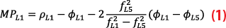
where ρ is the code measurement, ϕ are the carrier phase measurements, f the center frequencies of the navigation signals, and the subscripts L1 and L5 indicating the respective frequency band of the measurements. Subsequently, the obtained multipath estimate MPL1 was leveled to zero mean and an elevation mask of 5° was applied. The evaluations were done separately for the data collected at 2 m and 5 m above ground. To compare results for the two heights and two different smoothing time constants, the standard deviation of the multipath estimates per satellite as a function of its average elevation over the measurement period was calculated, and σair from the standardized airborne multipath model [2] was compared against the CMC data.
GBAS and SBAS Performance Evaluation
Finally, the observed airborne navigation performance of the GBAS and SBAS corrected positioning solutions are compared in terms of accuracy and protection level performance with a postprocessed reference trajectory. Using NovAtel’s GrafNav software, this reference is calculated as a differential carrier phase solution relative to a fixed installation on the rooftop of the university building located about four kilometers from the test area at Winterthur aerodrome. The GBAS and SBAS position solutions are computed using EUROCONTROL’s PEGASUS software [11], a toolset allowing the calculation of a variety of different GNSS-based navigation solutions compliant with the applicable aviation standards. Along with the position solutions, PEGASUS also outputs the respective Horizontal Protection Level (HPL). The protection levels for SBAS according to DO-229F [12] were used in this study. Based on specifications defined in DO-253D [2] horizontal protection levels for the GBAS positioning service (HPLGBAS,pos) were calculated as follows

with the transmitted integrity parameters for the GBAS message as the maximum of the nominal protection level (HPLH0), the faulted protection level (HPLH1) and the horizontal ephemeris error protection bound (HEB).

with Kffmd,POS being conservatively set to 10 according to the current standards [2]. However, this value is likely to change and be reduced, as also suggested in[8]. The parameter dmajor describes the size of the semi-major axis of the error ellipse, as defined in DO-253D. The faulted protection level HPLH1,j is calculated as

Where |.| refers to the absolute value function, Bhorz,j to the horizontal B-values being calculated on the basis of the transmitted GBAS message, Kmd,POSis the missed detection multiplier, which is set to 5.3 for the H1-case, and dmajor,H1is the semi-major axis of the error ellipse, differing from the nominal dmajor only by an inflated ground noise component accounting for the potentially faulted reference receiver. Finally, HEB is calculated as

with

where shorizontal,j is the horizontal s-value, xair is the distance between the GBAS reference point and the user, Pj is the ephemeris decorrelation parameter transmitted in the GBAS message, Kmd,e,pos is the missed detection multiplier for the ephemeris bound set to 4.1, and dmajorthe semi-major axis of the error ellipse. For all calculations of the error ellipses, nominal and standardized σair, which describe the residual noise and multipath errors for 100 seconds smoothed pseudoranges, were used. Finally, the horizontal protection levels for SBAS and the GBAS positioning service are compared. The Vertical Protection Level (VPL) performance is not shown in this study because no VPLs are defined for the GBAS positioning service as it was envisioned for large aircraft that would rely on barometric altimetry.
Results
Results were obtained by postprocessing GNSS and GBAS message recordings using the PEGASUS software tool. Postprocessing for GBAS was done twice. First, the standard smoothing time of 100 s was used. In a second run, the smoothing time was set to 10 s in the advanced PEGASUS settings.
GBAS Data Flight Track
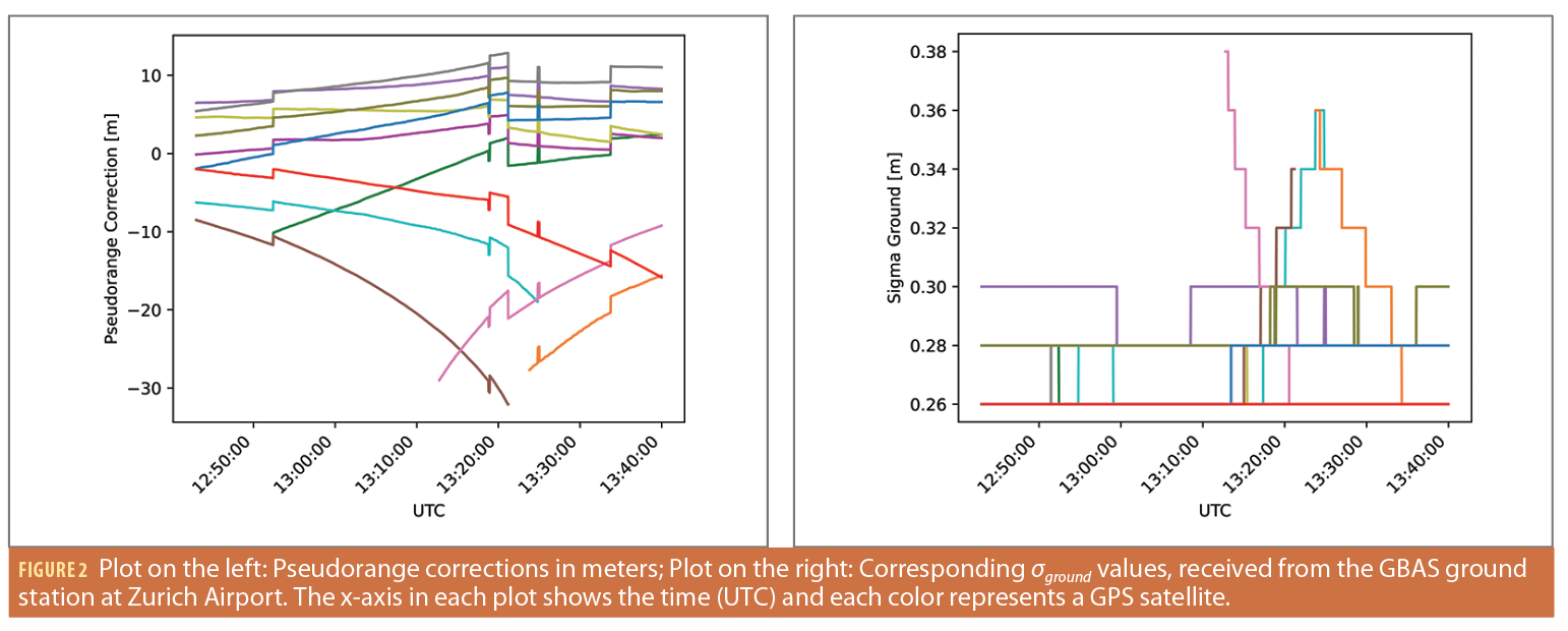
The GBAS message broadcast for the approach service from the operational station at Zurich Airport was received with a software defined radio and converted into the PEGASUS format for subsequent postprocessing. Figure 2, left, shows the broadcast pseudorange corrections (PRC) in meters. The corrections vary from about -33 m to just above +10 m. The very large corrections (in absolute terms) correspond to rising or setting satellites at low elevations. The sudden jumps in the corrections occur at epochs when a satellite is added or removed from the set of corrections. Figure 2, right, shows the broadcast values for σground, i.e., the residual error characterization associated with the pseudorange corrections. Typically, these vary between +0.26 m and +0.3 m, except for satellites at low elevations, shortly after rising or just before setting.
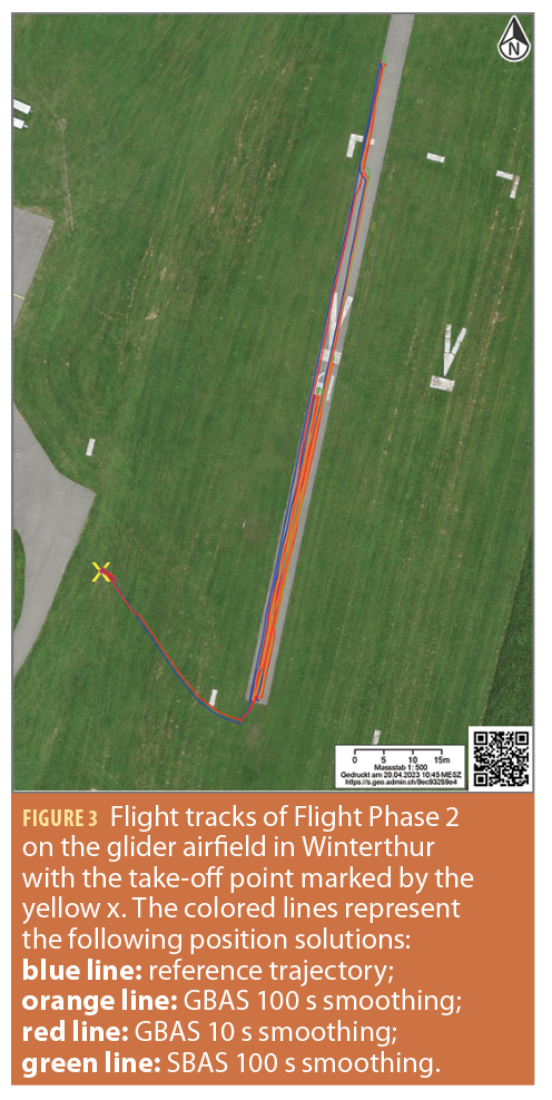
Figure 3 shows the ground track of Flight Phase 2 at an altitude of approximately 3.5 m above ground at the glider airfield in Winterthur. The following color codes illustrate the different position solutions:
• Blue line: Postprocessed differential carrier phase reference trajectory
• Orange line: GBAS
with 100 s smoothing
• Red line: GBAS
with 10 s smoothing
• Green line: SBAS
with 100 s smoothing
All evaluated flight tracks lie very close to each other and to the reference trajectory. The SBAS position solution (green line) is hardly visible as it lies below the other flight tracks. At the beginning of this flight phase from the drone’s take-off point (yellow cross) to the acceleration strip, only the blue and red line are visible. This is because with a smoothing of 100 s, the filter needs six minutes to converge. Therefore, 100 s of smoothing only outputs a position solution after six minutes of flight time, when the drone is already flying over the paved part of the runway.
Number of satellites used
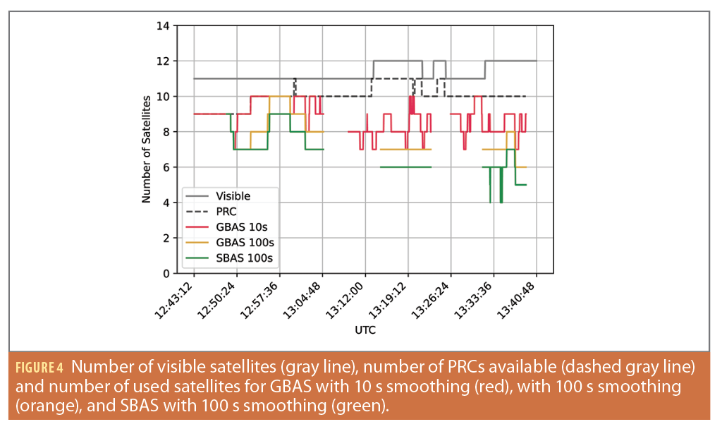
Figure 4 shows the number of satellites used throughout the flight for different processing modes. The left part, until about 13:04 UTC, shows the number of satellites from Flight Phase 1, where the UAV was hovering stationary at 15 m above ground. The middle part of the plot, between 13:09 UTC and 13:23 UTC, corresponds to Flight Phase 2 where the UAV was flown dynamically at medium velocity. The right part, from 13:26 UTC until approximately 13:39 UTC, refers to Flight Phase 3, where the UAV was flown dynamically at high velocity. Starting from the top of Figure 4, the solid gray line indicates the number of satellites visible at the time of the flight using a 5° elevation mask. This number corresponds to the theoretical maximum usable satellites. Note GBAS and SBAS only provide corrections for GPS, thus the number of satellites shown does not include visible satellites from other constellations. The dashed gray line illustrates the number of PRCs broadcast by the GBAS and is the maximum number of satellites for which GBAS corrections can be applied. The red and orange lines represent the number of satellites used in the GBAS solution with smoothing time constants of 10 s (GBAS10s ) and 100 s (GBAS100s), respectively. The green line depicts the number of satellites used in the SBAS solution with a smoothing time of 100 s (SBAS100s ). Because of the UAV’s attitude changes, the receiver loses track of satellites, therefore the number of used satellites in the different positioning modes is lower than the number of visible satellites. Moreover, the number of PRCs available is mostly one to two less than the number of visible satellites.
In Flight Phase 1, GBAS100s uses one to two fewer satellites than the number of PRCs available. GBAS10s uses mostly all satellites for which corrections are provided, except for a few times when one to two fewer satellites are used. Most of the time, more satellites are used in GBAS10s than in GBAS100s. SBAS100s uses two to four fewer satellites than the number of visible satellites.
In Flight Phase 2, where the UAV was moving at moderate speed with moderate attitude changes, GBAS100s uses seven out of 10 to 11 satellites for which corrections are provided. Due to the required waiting period for the smoothing filter convergence, the GBAS100s position solution is not available until 13:14 UTC, about six minutes after the beginning of this flight phase. The number of used satellites for GBAS10s varies between seven and 10 out of the available satellites. This means there were between one and four fewer satellites in use than the theoretical maximum. Again, GBAS10s generally use one to three satellites more than GBAS100s. SBAS100s always uses six out of 11 to 12 visible satellites and therefore one satellite less than GBAS100s.
In Flight Phase 3, where the drone was flown more dynamically and large attitude changes occurred, GBAS100s uses only between six and eight satellites out of the 12 visible and out of the 10 for which corrections were provided. Moreover, the GBAS100s solution only becomes available about six minutes into the test due to the wait time for smoothing filter convergence. In the GBAS10s solution, between one and three more satellites are used than in GBAS100s. Finally, the SBAS100s solution uses between five and seven satellites with three short drops to just four satellites.
Multipath Performance as a Function of Flight Altitude
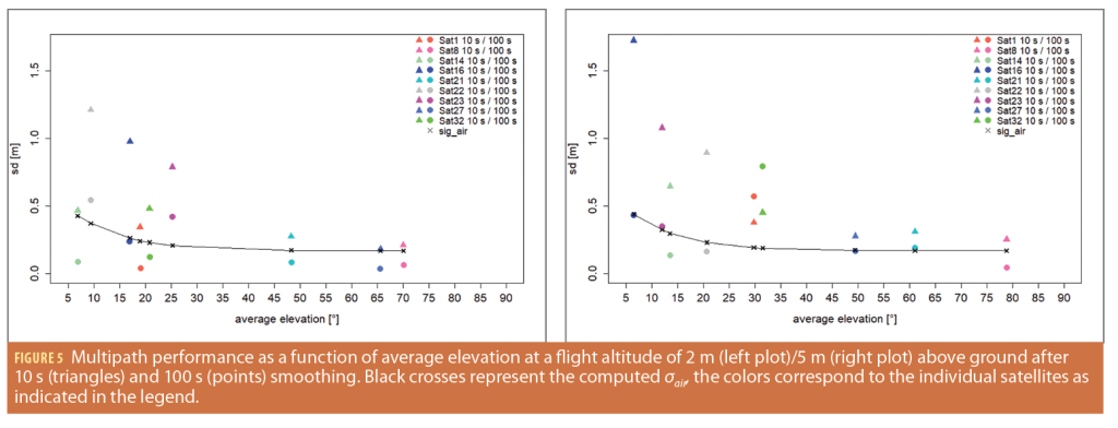
To analyze the differences in multipath in relation to the height of the drone above ground, the standard deviation of the observed multipath in a previous static hovering test was calculated per satellite and subsequently visualized as a function of the average elevation during the few minutes where data was collected. The left plot in Figure 5 shows the standard deviations of every satellite with smoothing time constants of 10 seconds (triangles) and 100 seconds (points) for every average elevation angle of each satellite while hovering at an altitude of 2 m above ground. The standardized airborne multipath model (black crosses and black line) is shown for comparison purposes. The same data is shown for the flight period at 5 m above ground in Figure 5.
In the case of hovering at 2 m above ground (plot on the left), it can be seen that standard deviation after 10 seconds of pseudorange smoothing is always significantly larger than after 100 seconds of smoothing. Also, a decreasing trend of the standard deviations with increasing average elevation angles is visible, especially in the case of 10 s smoothing. The 100 s smoothed multipath estimates are mostly in line with the standardized airborne multipath models, while the data using only 10 s of smoothing significantly exceeds the curve. For an altitude of 5 m above ground (plot on the right), the generally higher values after 10 seconds of smoothing (with the exception of Sat 1 and Sat 32) as well as the decreasing trend of the standard deviations with increasing satellite elevation are visible again. In comparison to the multipath performance at 2 m above ground, the standard deviation of the satellite at just over 5° elevation (Sat 16) after 10 seconds of smoothing (triangle in dark blue) is significantly larger. Most other satellites show a more modest increase in the standard deviations but indicate an increasing trend compared to the data from just 2 m above ground.
Horizontal Protection Level Performance (GBAS /SBAS)
To evaluate the potential benefits of applying GBAS corrections during a drone flight, the HPL of the GBAS and the SBAS positioning service after 100 s of smoothing were compared. GBAS HPL with 10 s of smoothing was not considered for this comparison because the filter time constants of the pseudorange and the PRCs must be the same, otherwise there could be an error buildup in the filter that would distort the navigation solution. The GBAS position solution with 10 s smoothing is only used to show the influence of the smoothing time constant on the number of satellites used.
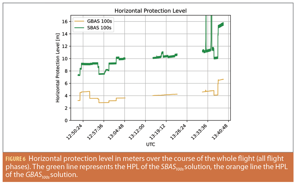
Figure 6 shows the comparison of the GBAS100s and SBAS100s HPLs over the course of all three flight phases. The green line illustrates the HPL SBAS100s, while the orange line depicts the HPL GBAS100s. Throughout the flight, the HPL GBAS100s stays well below the HPL SBAS100s. Whereas the HPL SBAS100s varies between approximately seven and just over 10 meters in Flight Phase 1 (12:50 until 13.04 UTC), the HPL GBAS100s rises shortly up to nearly five meters at the beginning of the flight. After about four minutes, the HPL decreases and stays between 2.8 and 3.6 meters for the remainder of Flight Phase 1.
In Flight Phase 2 (13:14 until 13:23 UTC), both HPLs are higher than in Flight Phase 1 and increase throughout the flight. The HPL SBAS100s starts at 10 meters and increases up to about 10.8 meters with one jump up to over 11 meters. The HPL GBAS100s rises steadily from 4.0 to 4.3 meters.
In Flight Phase 3, a significant jump in the HPLs can be seen. The HPL GBAS100s starts at about 4.6 meters and increases slowly. At 13.35 UTC, a drop in the HPL down to just above four meters is visible. This is because the number of satellites used increases from seven to eight. After about two minutes, the number of satellites used in the GBAS100s solution decreases to only six and the corresponding HPL jumps to about 6.5 meters. The HPL SBAS100s exhibits an even bigger jump from 10 to 15 meters. Moreover, the HPL SBAS100s has several sudden jumps in the HPL, e.g., at 13:32 UTC to over 16 m, or at 13:34 UTC up to 200 m. The reason for these large degradations is the receiver loses or incorrectly receives SBAS messages. If ionospheric corrections cannot be computed, the positioning mode switches from Precision Approach (PA) to Non-Precision Approach (NPA) with much larger corresponding protection levels. This effect also may be caused by the UAV’s dynamic maneuvering and the associated difficulty in tracking and correctly decoding SBAS messages. The horizontal protection levels are generally larger in Flight Phases 2 and 3, where the UAV was flown dynamically. This corresponds to the lower number of satellites used. Finally, the SBAS protection levels show a certain oscillating behavior in the range of a few decimeters. This is caused by the degradation factor associated with the fast corrections until the next valid set of corrections is used and applied.
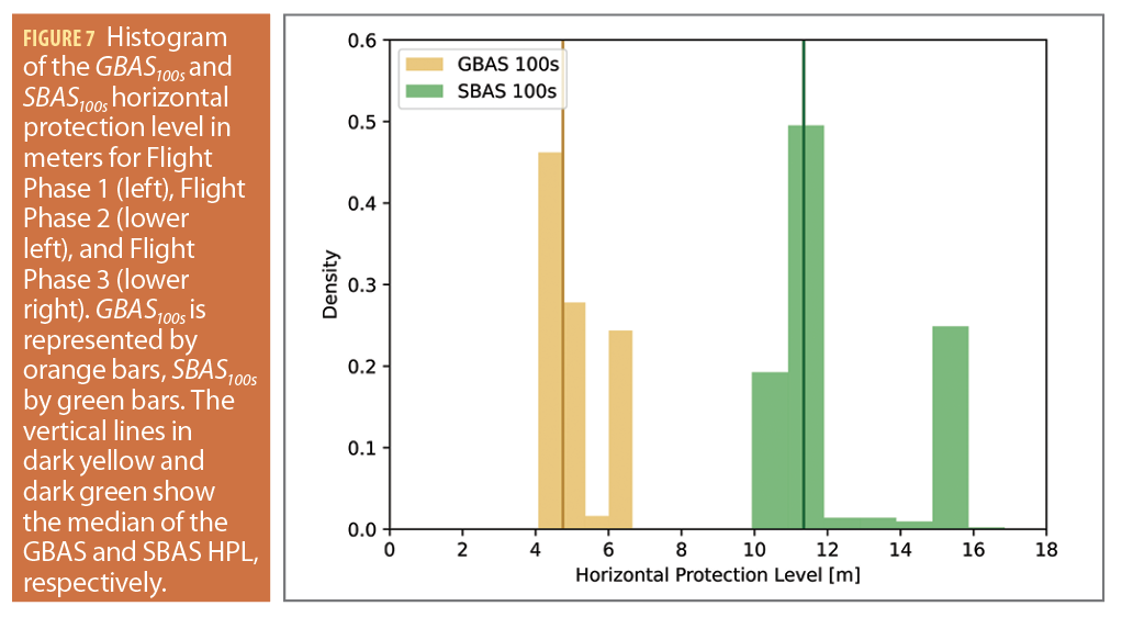
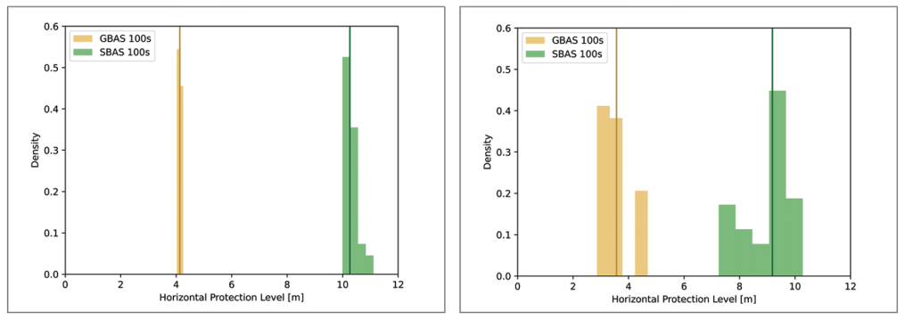
Figure 7 shows the histograms of the protection levels of GBAS100s and SBAS100s for Flight Phases 1, 2 and 3. The GBAS protection level after 100 s smoothing is illustrated by the orange bars and the SBAS protection level after 100 s smoothing by the green bars. The vertical lines in dark orange and dark green show the median of the respective HPL. In Figure 7, the HPLs for GBAS and SBAS are
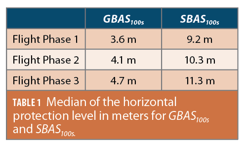
visualized from from top left to lower right for Flight Phases 1, 2 and 3, respectively. In all flight phases, the GBAS protection level is substantially lower than the SBAS protection level. This is confirmed by the median values in Table 1. The median of HPL GBAS100s ranges between 3.6 and 4.7 m whereas the HPL SBAS100s lies between 9.2 and 11.3 m.
Comparison to Reference Trajectory
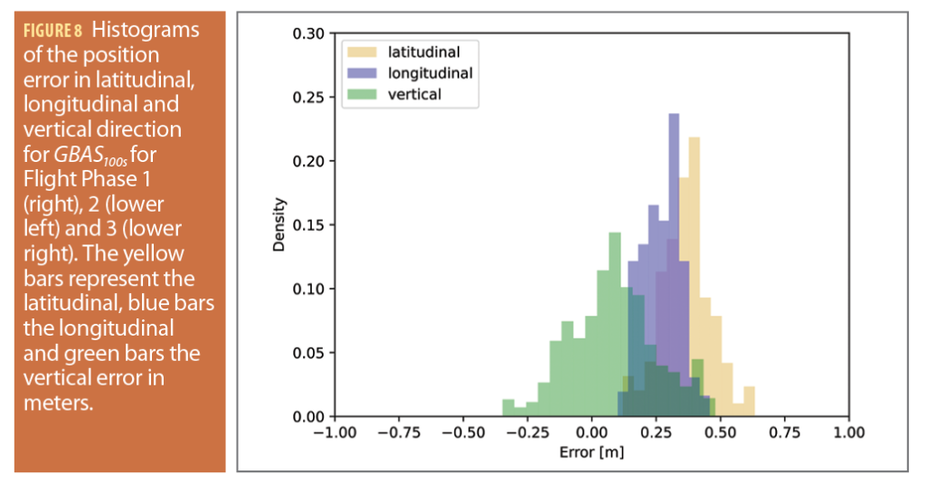
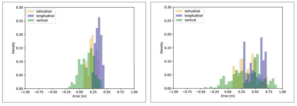
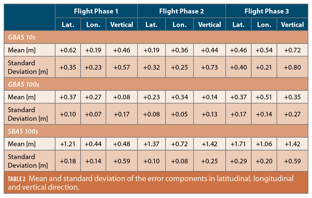
In the previous sections, multipath as well as the protection level performance were evaluated. Here, the accuracy of the GBAS and SBAS augmented solutions is assessed through a comparison with a postprocessed differential carrier phase reference trajectory. Figure 8 shows the histograms of the position error in latitudinal, longitudinal and vertical direction for GBAS100s for Flight Phases 1, 2 and 3, from top left to lower right. The errors in Flight Phase 1 lie mostly between -0.4 and +0.6 meters with the vertical error being the most and the longitudinal error the least scattered. In Flight Phase 2, the dispersion is generally lower, with values mostly varying between -0.2 and +0.5 m. Again, the error in vertical direction has the widest and the error in longitudinal direction the narrowest spread. In Flight Phase 3, the error scatter in the vertical direction is significantly more pronounced than in the flight phases before, with most of the values ranging from -0.4 to +0.9 m. The spread of the latitudinal and longitudinal errors is smaller, with values varying from 0.0 to +0.75 m. The mean and standard deviation of the errors in the three dimensions, the three flight phases, and the three different processing modes are summarized in Table 2. When comparing the mean errors of GBAS10s and SBAS100s against the errors of GBAS100s, it is clear SBAS100s has the highest mean for all error directions and flight phases. However, the standard deviations of SBAS100s are mostly lower than GBAS10s.
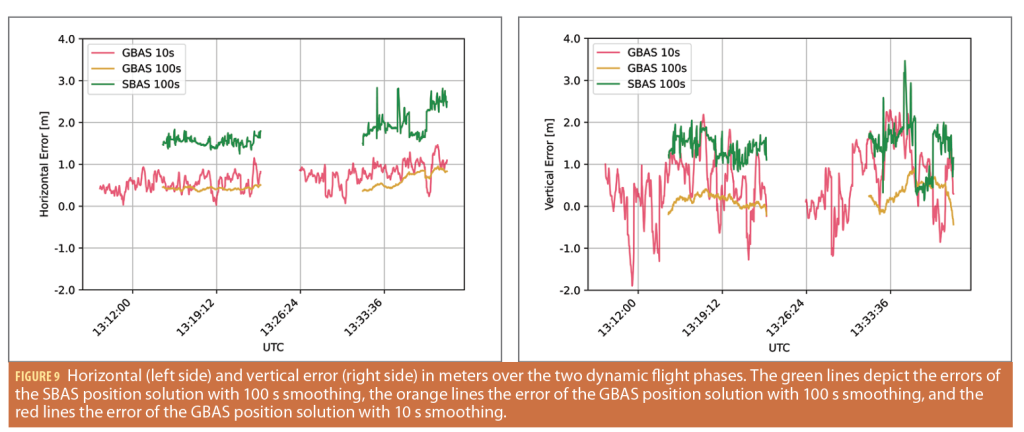
Figure 9 depicts the horizontal and vertical errors over the time of the dynamic flight phases in meters. The horizontal error is shown on the left side of the plot and the vertical error on the right. The red line represents the GBAS10s solution errors, the orange line the GBAS100s solution errors and the green line the SBAS100s solution errors.
The GBAS10s horizontal errors range from 0.0 to +1.2 meters in Flight Phase 2 and +0.1 to +1.5 m in Flight Phase 3. The GBAS100s solution contains errors ranging from +0.3 to +0.5 and +0.4 to +1.0 m in Flight Phase 2 and 3, respectively. In comparison to GBAS10s, it is obvious the shape of the curve is much smoother, with fewer and smaller fluctuations. The SBAS100s solution errors have a significant offset compared to the other two position solutions. The error values range from +1.3 to +1.8 m in Flight Phase 2 and from +1.5 to +2.8 m in Flight Phase 3. The shape of this curve is smoother than the one of GBAS10s but has more fluctuations than GBAS100s, especially in Flight Phase 2. The vertical errors lie in a greater range of values, especially for GBAS10s and SBAS100s. The curve of GBAS10s varies between -1.9, +2.2 meters in Flight Phase 2 and -1.2, +2.3 meters in Flight Phase 3 and again has frequent fluctuations. In contrast, the GBAS100s has fewer variations and a narrower range of values (-0.2 to +0.4 m and -0.4 to +0.9 m in Flight Phase 2 and 3, respectively). In Flight Phase 2, the SBAS100s errors are above the GBAS10s position solution errors most of the time with values ranging from +0.8 to +2.0 m. In Flight Phase 3, SBAS100s errors have strong fluctuations, similar to GBAS10s. These values vary between +0.1 and +3.5 meters. The three peaks in the vertical error (up to +2.6, +3.5 and +2.9 meters, respectively) correspond to the times where the number of satellites used in the SBAS position solution decreases to just four satellites for short periods.
Flight Profile, Maneuvering and Equipment
The flight was conducted at a height of 15 m (static hovering) and 3.5 m (dynamic flight) above ground, which are rather low altitudes. Flights conducted at higher altitudes may be less susceptible to impacts from multipath and would be preferrable from that perspective. In general, a UAV’s dynamics and attitude changes are much more significant than large transport aircraft. Furthermore, the antenna and receivers used on UAVs tend to be smaller and often show inferior performance than ones employed in operational and certified avionics on board large aircraft. This may lead to larger errors stemming from increased noise and potentially larger errors induced by antenna group delay [13].
Number of Used Satellites and Smoothing Time
Figure 4 suggests a significant difference between the 10 s (GBAS10s) and 100 s smoothed GBAS position solutions (GBAS100s), as GBAS100s uses one to two satellites (in a static scenario) and up to three satellites (dynamic flight) less than GBAS10s at the same time. Dynamic maneuvers may cause large and sudden changes in the UAV’s attitude and lead to frequent loss of individual satellite tracking, as the smoothing filter needs to be re-initialized. After re-initialization of the smoothing filter, it takes 3.6 times the smoothing time constant for the filter to converge [9]. Thus, the position solution is calculated based on fewer satellites leading to increased errors and larger protection levels due to the weaker satellite geometries. Currently, avionics manufacturers usually re-include satellites much quicker but inflate the corresponding σair for that satellite. However, PEGASUS conforms to the minimum operational performance requirements and thus waits for filter convergence before re-inclusion of the satellite into the position solution.
For instance, in the case of 100 s of smoothing, a satellite has to be tracked continuously for six minutes before it is re-included. When setting the smoothing time filter constant to 10 s, PEGASUS re-incorporates the lost satellites after just 36 seconds, leading to more available satellites for navigation purposes. For operational purposes, however, the use of this shorter smoothing time constant would need more detailed research because the mismatch in smoothing time constant between the airborne measurements and the PRCs generated on the ground can lead to build-up of differential errors that must be avoided. Furthermore, the transient phase of the smoothing filter must be better understood and properly bounded so it might be possible to re-include satellites faster with appropriately inflated integrity parameters. Trying to avoid losing track of satellites to begin with is another mitigation method. While the GNSS antenna is usually rigidly attached to UAVs, placing the GNSS antenna on a gimbal to decouple it from the vehicle’s dynamic movement could help maintain more stable tracking.
Multipath Performance
The amount of residual multipath in the position solution largely depends on the amount of multipath affecting the measurements in the first place and subsequently on the smoothing filter used to reduce the impact. While residual errors on pseudoranges after 100 s of smoothing are well in line with the standardized airborne multipath models, the data using only 10 s of smoothing considerably exceeds the models and a significant amount of residual noise and multipath persists in the position solution. These findings are consistent with the airborne multipath assessments for UAVs conducted by [5] and the discussion about smoothing filter convergence by [14]. Most likely, the UAV airframe itself does not cause reflections more severe than a large transport aircraft. However, UAVs come in various shapes and sizes so such a claim should be investigated for each type of vehicle.
Typical altitudes at which UAVs operate tend to be high enough that the mounted GNSS antenna is not influenced by ground reflections. However, when operating close to the ground, especially during take-off and landing, this might not be true, meaning more multipath can affect the airborne receiver. In general, it seems to be reasonable to assume the σair values derived for large transport aircraft can also bound multipath errors in dynamic UAV operations. However, the variety of UAVs, GNSS antenna and receiver installation and performance can differ significantly. Besides that, the potential operation areas for UAV are wide. Thus, it is challenging to generate and use a one-size-fits-all model for airborne multipath that holds in all scenarios.
GBAS and SBAS Protection Level Performance
In general, the proposed approach to receive and decode GBAS messages at one location (in this case at Zurich Airport) and apply them at another location for users who cannot directly receive the VDB data broadcast of the ground station worked well. However, safely bounding residual errors is a critical step when using GNSS for safety-critical applications. This is achieved by calculating protection levels. GBAS provides locally generated corrections and integrity parameters, while SBAS provides correction and integrity parameters on a continental scale. In close proximity to the GBAS ground station, this study confirmed the protection levels for GBAS are significantly smaller than those bounding the residual SBAS errors. In the dynamic flight phases, the HPL for GBAS100s was roughly on the order of four meters, while for SBAS100s these values were on the order of roughly 10 m. In the static flight phase, the corresponding HPLs were slightly smaller. The distance between our UAV flight test and the GBAS at Zurich Airport was approximately 15 km, both rather close to the airport and within the specified GBAS service area, where good performance could be expected.
Finally, protection levels depend on the geometry of the satellites available for the calculation of a position solution. A drone’s large attitude angles and frequent attitude changes in flight together with the necessary smoothing and time for the smoothing filter to converge reduce the number of available satellites and thus impacts protection level performance. The situation may further worsen for scenarios where a UAV is landing and part of the sky is blocked by obstacles near the landing site. Using just 10 s smoothing in PEGASUS showed the potential benefit in terms of having more satellites available for longer periods. However, the standardized error models developed to bound the residual errors in steady state after filter convergence using a time constant of 100 s do not bound the residual errors after just 10 s smoothing. For that reason, no meaningful protection levels for 10 s smoothing could be calculated.
Positioning Accuracy
Another important performance parameter is, of course, the accuracy of the position solution. For determining the GBAS positioning errors, we calculated a reference trajectory and compared the GBAS and SBAS results against it. The errors for all three different processing methods remained well within the range of expected errors for an augmented code-based position solution. When comparing the accuracy of GBAS10s and GBAS100s significantly more noise and multipath remains after 10 s than after 100 s smoothing. The low-frequency error components, however, are comparable. The SBAS solution generally exhibits larger errors than the GBAS solutions, which also can be expected as GBAS provides local corrections and tends to correct more of the residual errors when users are operating reasonably close to the ground station.
Conclusions
In this study, we presented a proof of concept for using GBAS corrections from an operational ground station for applications other than guiding large aircraft on final approach. In our case, GBAS corrections were used for navigating a UAV. One main challenge is the ability to receive broadcast corrections as VHF communications near line-of-sight must be given to ensure reception. As this is typically not the case for UAV operations, we explored receiving, decoding and forwarding GBAS messages by other means, such as via the cellphone network. Frequent and significant changes of the UAV’s attitude angle makes it difficult to track satellites and required a re-initialization of the smoothing filter. Convergence of the smoothing filter may be time consuming, especially when using a 100 s smoothing filter, as required when using GBAS corrections. Therefore, for such operations, it is desirable to re-include satellites faster into the position solution so satisfactory performance can be achieved. For this issue, using multiple constellations and therefore having significantly more satellites available would greatly improve the performance and reduce the impact of losing satellites. Another way to avoid loss of tracking would be to mount the GNSS antenna on a gimbal on top of the UAV, so the antenna is not tilted with the aircraft when maneuvering.
Acknowledgements
The results presented in this paper were developed within a project funded by Swiss FOCA under grant number SFLV2019-038. The authors would like to thank FOCA for their funding and support for the topic.
This article is based on material presented in a technical paper at ION GNSS+ 2022, available at ion.org/publications/order-publications.cfm.
References
[1] RTCA (2017a), GNSS-based precision approach local area augmentation system (LAAS) signal-in-space interface control document (ICD) (DO-246E). https://www.rtca.org/
[2] RTCA (2017b), Minimum operational performance standards for GPS local area augmentation system airborne equipment (DO-253D). https://www.rtca.org/
[3] Pullen, S., Enge, P., & Lee, J. (2013a). High-integrity local-area differential GNSS architectures optimized to support UAVs (Unmanned Aerial Vehicles). Proceedings of the 2013 International Technical Meeting of The Institute of Navigation
[4] Pullen, S. (2013b). Managing separation of unmanned aerial vehicles using high-integrity GNSS navigation. Proc EIWAC 2013, 19-21.
[5] Kim, M., Kim, K., Lee, D. K., & Lee, J. (2015). GNSS airborne multipath error modeling under UAV platform and operating environment. Journal of Positioning, Navigation, and Timing, 4(1), 1-7. https://doi.org/10.11003/JPNT.2015.4.1.001
[6] Murphy, T., Harris, M., Geren, P., Pankaskie, T., Clark, B., & Burns, J. (2005, September). More results from the investigation of airborne multipath errors. Proceedings of the 18th International Technical Meeting of the Satellite Division of The Institute of Navigation (ION GNSS 2005) (pp. 2670-2687).
[7] Circiu, M. S., Caizzone, S., Felux, M., Enneking, C., Rippl, M., & Meurer, M. (2020). Development of the dual‐frequency dual‐constellation airborne multipath models. NAVIGATION, 67(1), 61-81. https://doi.org/10.1002/navi.344
[8] Jochems, S., Felux, M., Schnüriger, P., Jäger, M., & Sarperi, L. (2022, January). GBAS use cases beyond what was envisioned–drone navigation. Proceedings of the 2022 International Technical Meeting of The Institute of Navigation (pp. 310-320), https://doi.org/10.33012/2022.18213
[9] EUROCAE (2019), Minimum operational performance standard for global navigation satellite ground based augmentation system ground equipment to support precision approach and landing (ED-114B). https://www.eurocae.net/
[10] Hatch, R. (1983). The synergism of GPS code and carrier measurements. International geodetic symposium on satellite doppler positioning (Vol. 2, pp. 1213-1231).
[11] EUROCONTROL (n.d). PEGASUS. Retrieved April 27, 2023, from https://www.eurocontrol.int/tool/pegasus
[12] RTCA (2020), MOPS for global positioning system/satellite-based augmentation system airborne equipment (DO-229F). https://www.rtca.org/
[13] Caizzone, S., Circiu, M. S., Elmarissi, W., Enneking, C., Felux, M., & Yinusa, K. (2019). Antenna influence on GNSS pseudorange performance for future aeronautics multifrequency standardization. NAVIGATION, 66(1), 99-116. https://doi.org/10.1002/navi.281
[14] Circiu, M. S., Felux, M., Belabbas, B., Meurer, M., Lee, J., Kim, M., & Pullen, S. (2015, September). Evaluation of GPS L5, Galileo E1 and Galileo E5a performance in flight trials for multi frequency multi constellation GBAS. In Proceedings of the 28th International Technical Meeting of The Satellite Division of the Institute of Navigation (ION GNSS+ 2015) (pp. 897-906).
Authors
Sophie Jochems obtained a Bachelor of Science in Aviation at the Zurich University of Applied Sciences (ZHAW) in 2019. Since July 2021, she has worked as a research assistant at the Center for Aviation at the ZHAW within the research group Aviation Infrastructure. Her research focus lies on satellite navigation and its use in the field of drone navigation.
Valentin Fischer obtained a Bachelor of Science in Aviation at the Zurich University of Applied Sciences (ZHAW) in 2022. In fall 2022, he started his Master of Science in Aviation at ZHAW. Since then, he has worked as a research assistant at the Center for Aviation within the research group Aviation Infrastructure. His research focus lies on satellite navigation and aviation infrastructure topics.
Michael Felux is a senior lecturer and leader of the Aviation Infrastructure Team in the Centre for Aviation at the Zurich University of Applied Sciences. He holds a PhD in Aerospace Engineering and has worked on safe and secure navigation for aviation for 12 years.
Michael Jäger received a Master of Science in Engineering with specialization in Information and Communication Technologies from Zurich University of Applied Sciences (ZHAW), Switzerland, in 2010. He has over 10 years of experience in industrial R&D and has worked as a research assistant for wireless communications at Zurich University of Applied Sciences since 2019. His field of research includes radar and LiDAR systems, wireless localization and software defined radio applications.
Luciano Sarperi has over 15 years of experience in R&D in the telecommunications sector and has been a lecturer in Wireless Communications at the Zurich University of Applied Sciences (ZHAW) since 2017. His interests in applied R&D include wireless localization, IoT systems, mobile communications and software defined radio applications.
Natali Caccioppoli studied radio-electronic navigation, and telecommunication engineering, at Universitá degli Studi di Napoli Parthenope, Italy, holding two laurea degrees (cum laude). In 2003, he was appointed as Fellow Researcher at the “G. Latmiral” Engineering School granted by the Italian aerospace research centre (CIRA) working on GNSS Signal Processing. Since October 2008, he has worked as a GNSS Operational Validation Expert Consultant at EUROCONTROL Innovation Hub (France) in the domain of GNSS aviation applications (SBAS, GBAS, A/RAIM, RFI). Since June 2017, he has earned the IATA AvMP Designation issued by Stanford University and IATA.
![Some of the equipment that makes up Indra’s GBAS; Image courtesy Indra[87]](https://insidegnss.com/wp-content/uploads/2025/11/Some-of-the-equipment-that-makes-up-Indras-GBAS-Image-courtesy-Indra87-150x150.jpg "Indra Navia Leading the Evolution Towards Dual-Frequency GBAS")


