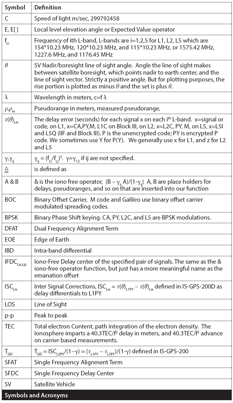
 Symbols and Acronyms
Modernized GPS satellites give civil users the ability to achieve dual L1/L2 PY accuracy using dual L1CA/L2C ionosphere-free measurements and, with IIF satellites, dual L1/L5 signals. Because broadcast GPS ephemeris data is based on an ionosphere-free pseudorange calculated from dual L1PY/L2PY measurements and the civil signals are not all perfectly aligned to it, new broadcast parameters and a new modernized dual-frequency algorithm are needed in order to align new signals with the dual L1/L2 PY signal.
Modernized GPS satellites give civil users the ability to achieve dual L1/L2 PY accuracy using dual L1CA/L2C ionosphere-free measurements and, with IIF satellites, dual L1/L5 signals. Because broadcast GPS ephemeris data is based on an ionosphere-free pseudorange calculated from dual L1PY/L2PY measurements and the civil signals are not all perfectly aligned to it, new broadcast parameters and a new modernized dual-frequency algorithm are needed in order to align new signals with the dual L1/L2 PY signal.
New inter-signal correction (ISC) broadcast parameters and the modernized dual-frequency algorithm were published in 2004 in the unclassified interface specification documents IS-GPS-200D and IS-GPS-705. (Note: Originally, IS-GPS-200 was an interface control document, ICD-GPS-200, but changed to be an interface specification IS-GPS-200 for rev D and beyond.) There are more L1/L2 IIR-M and IIF satellites now broadcasting civil navigation (CNAV) messages along with inter-signal corrections (MSG 30), but there will be more L1/L5 satellites in the long term when Galileo and other GNSS systems become options.
The parameters used in this new dual-frequency algorithm are based on two assumptions: 1) the antenna delays are approximately constant over the main beam, and 2) any electrical changes are slowly varying such that they can be treated as constants during data set upload intervals. However, published research (see references 3, 5, and 6 in the Additional Resources section at the end of this article) has shown delay variation across the main beam due to space vehicle (SV) antenna anisotropy — that is, directionally dependent differences in physical properties of the antenna (defined in IS-GPS-200F) — and thus needs to be considered for future navigation performance.
This article will examine the ISC constancy approximations and examine two techniques for measuring ISC values that will be broadcasted and explain their pros and cons. The first technique measures the ISCs using code and carrier phase information. The second technique re-arranges the modernized dual-frequency correction algorithm in terms of the new parameterization of intra-band differentials (IBDs). Further, this article will provide methods to convert between ISCs and IBDs.
With these explanations, receiver designers will understand a) how the measurement technique used enables constant ICS values to achieve accurate dual L1CA/L2C point positioning consistent with European differential code biases on the 0.1–2 nanosecond level [reference 3.5], b) the physics behind the new ICD term of SV antenna anisotropy, and c) understand some of the trade-offs such as L1/L2 vs. L1/L5 alignment errors based on ISC accuracy in the new modernized dual frequency correction algorithm.
After an introductory overview, the article is organized into the following sections: defining and modeling pseudorange alignment errors; ISCs, iono-free delay centers (IFDCs), and their impact on navigation; alignment and measurement algorithms; measurement data; and conclusions and recommendations.
All technical appendices can be found in the Additional Information section at the end of this article.
Overview
The left side of Figure 1 shows the legacy and modernized ionospheric correction equations from IS-GPS-200. The right side of Figure 1 shows our alternative formulation. The original 1991 IS-GPS-200 equations (1) and (2) in Figure 1 combines L1PY and L2PY pseudorange measurements (ρm) into a single pseudorange that is “free” of any 1/f2 ionospheric delay. However, a new ionosphere-free equation (3) is needed to account for the multiple carrier frequencies and for SV-specific signal alignment errors in the new L2C and L5I and L5Q signals.
Due to variations within the SV equipment, each signal has a unique delay τLix, where i=1,2,5 for L1, L2, and L5, and x = the corresponding code on that carrier. (Note: each different signal or code, x, such as CA, P, and M on L1, L2C, P, M on L2, L5I&L5Q on L5, and so on, is a PRN spreading code, and we will refer to each of these as either signals or codes. On a GPS satellite, all signals/codes are assigned the same PRN number. Each satellite is assigned an SVN number and the PRN to SVN mapping can change. The sem file format supports identification of the PRN, SVN, and block type, as documented online here. Technically, signals are the carrier with modulated code, but within the literature, signal and code have both been used interchangeably.)
ISCs (IS-GPS-200D, circa 2004) are defined in Equation (4) as delay differentials between all signals relative to L1PY. Each SV has its own unique set of ISCs.
For those familiar with the earlier versions of IS-GPS-200, the legacy scaled group delay parameter TGD can be expressed in terms of ISCL2PY as shown in Equation (5). The original frequency scaling factor γ is now γij as shown in Equation (6) where i and j refer to the two frequencies used in the delay differential. Equation (3) reduces to equation (1) by inserting equations (4 through 6) into (3) and for Lix using i=1 x=PY for L1PY and for Ljz using j=2 and z=PY for L2PY.
We will use the symbol “&” to represent the ionosphere-free operator defined by equation (1). For the purposes of this article, we will focus on L1 & L2 or L1 & L5 pairs because L2 & L5 combinations are not numerically stable.
Equation (3) doesn’t preclude ISCLix parameters that vary with SV boresight angle θ (SV antenna anisotropy). However, the current modernized navigation messages support only constant ISC values. As we will show, antenna anisotropy can challenge this assumption. In addition, ground monitoring stations have difficulty measuring non-constant ISC values unless they can see the full antenna pattern.
We have developed an alternative formulation of Equation (3) that solves these difficulties, expressed as equations (7-8) on the right side of Figure 1. We begin by factoring equation (3) into a new form by moving TGD into the numerator, setting i=1 and j=2 or 5 for L1 & L2 or L1 & L5, and grouping the TGD term with ISCLjz.
The terms in the square brackets become the IBDs (intra-band delays). IBDs as a function of ISCs is defined by equation (8) as:
Examining equations (8), (8a), and (8b), for L1 and L2 we notice that the IBDs for j=1,2 are intra-band differences between any code on the jth L band and the PY code found within that L-band. Within a single carrier, the receive antenna, ionosphere, and the line-of-sight (LOS) delays are equal and will cancel out, making IBDs easier to measure. More importantly, the L1 and L2 IBDs are typically constant across the SV antenna aperture’s main beam when all civil signals are measured with delay lock loops (DLLs) using ICD 200F–specified tap spacings (Appendix B). Even if a ground site making the IBD measurements can only see a portion of an SV’s antenna, it can accurately measure the main-beam IBDs.
When j=5, complications arise. Although we don’t get a physical L5 IBD (8c), it behaves as if there is an effective L5PY reference (8d). The L5 IBD, equation (8c), is free of ionospheric contamination because the (1 − γ15) / 1 − γ12) scaling converts the L1-L2 iono error into an L1-L5 iono error. However, the L5 IBDs will vary with boresight angle.
Equation (8) has one other significant property: by using TGD, all IBD values can be converted into ISC constants compatible with the current CNAV messages on L2 and L5 and broadcast ephemeris assumptions. This allows single frequency users to align their one L-band measurement to the dual L1PY&L2PY ionosphere free pseudorange. The rest of this article, along with its on-line technical appendices, will rigorously derive and demonstrate the foregoing assertions.
Defining and Modeling Pseudorange Alignment Errors
A physical model of the satellite’s differential delays is developed using IS-GPS-200 notation. Because our focus is on the SV electronics and SV antenna, SV boresight angle θ is more appropriate than user elevation angle E (90-degree elevation is zero degree boresight, and 5 degree elevation is SV edge-of-earth beam-width of θ~13.9°, Appendix A).
Physical Model. Figure 2 shows the SV, ionosphere, and troposphere that add delays to the measured pseudorange. Because troposphere, SV clock, and receiver antenna delays errors are typically removed by look-up tables or broadcast algorithms, our measurement model, equation (9), simplifies to:
Equation (9) contains the desired line of sight pseudorange ρLOS, the signal specific SV equipment delays τLix(θ) which are functions of each L band and each signal, the ionosphere’s total electron content 40.3*TEC/f2Li contribution, and receiver noise nLix. Equation (9) is used to assess how SV-unique equipment delays τLix(θ) affect both single- and dual-frequency navigation. The speed of light c in equation (9) converts delay in seconds into meters. (Note: We will sometimes show a delay quantity being an explicit function of boresight angle. Other times, it is not shown in order to shorten the equations. In general, all of the delay parameters are a function of SV boresight and SV azimuth angle. In general, there is circular symmetry; so, the azimuth dependence is usually negligible. However, it is prudent to continually check this assumption.)
IS-GPS-200 Model. Paragraph 3.3.1.7 of IS-GPS-200 defines SV equipment delay as the “delay between the signal radiated output of a specific SV (measured at the antenna phase center) and the output of that SV’s on-board frequency source.” Paragraph 30.3.3.3.1.1.1 introduces SV signal–dependent equipment delays in terms of inter-signal corrections, ISCLix, defined as differential delays relative to the L1PY delay: τL1PY − τLix.
Figure 3 is a schematic representation of SV equipment delay as the accumulation of delays from the code generators, modulators, transmitters, tri/quadraplexors, and the SV antenna emanation point. (IS-GPS-200 refers to this point as the phase center.) If there is SV antenna anisotropy, the SV equipment delay is denoted as a function of boresight angle θ, τLix(θ). Red, blue, and green are used to color code L1, L2, and L5 frequency bands. Black lines represent the ISCs for each differential of τL1PY − τLix.
Emanation Point Using Phase and Delay Measurements. GPS signals are spread-spectrum codes modulated on to an L-band carrier. When traversing the ionosphere or an electrical network, the group delay of the code/envelope can be different than the delay of the carrier. Code delay is a shift in the signal envelope (i.e., group delay) and is measured in seconds. Phase delay is a shift in the carrier and is measured in units of radians. (Reference 1.5 in Additional Resources provides links to animations of phase and group delay independence.) Pseudorange is affected by code delay. Integrated carrier phase (called delta range in the literature) is affected by phase delay. When the SV equipment delays code and carrier by different amounts, the code and carrier emanation points can be different.
The antenna phase center is defined at the origin of the radius-of-curvature best fit to the far-field lines of phase and is the emanation point for the carrier. (In practice, the best fit to the radius of curvature lines of constant phase or delay is not a point but a region. The radius of the region should be much smaller in size than the smallest error of concern in the PPS performance standard. In the current precise positioning system or PPS standard, the miscellaneous SV error terms and/or group delay stability in the signal-in-space error budget is 0.6 meter or 0.2 nanosecond, 95 percent; so, an emanation point with an uncertainty radius of 0.2 nanosecond would be a reasonable good emanation tolerance size to start with.)
The notion of defining a best fit radius-of-curvature is also needed for lines of far-field constant group delay. When a receiver combines code and carrier ranging information, the individual emanation points of the pseudorange and carrier matter. This leads us to define an antenna delay center (DC) which locates the emanation point of the pseudorange. Although no application required the concept of an antenna delay center at the time the 1979 IEEE antenna standard was drafted, the concept has since been acknowledged (for example, see Additional Resources references 1.2 and 6.1). We will use the technically more precise “delay center” when referring to what IS-GPS-200 calls “phase center” as applied to code-only navigation. Appendix B (available online) summarizes the metrics used to measure “group delay.”
Not only do we need the concept of delay centers for individual signals, but we also need them for any ionosphere-free (IF) pair that we want to use for navigation, hence, iono-free delay center (IFDC). Aligning both single-frequency pseudoranges as well as ionosphere-free pseudoranges to the original L1PY and L2PY ionosphere-free pseudorange was the purpose of the introduction of ISCs into IS-GPS-200. Mathematically, ISCs allow alignment errors to be expressed in terms of differentials. In practice, we will show that a) IBDs are easily measured differential delays, b) pairs of IBDs physically represent the alignment errors between the blended emanation point of any new pair of signals relative to the blended emanation point of L2PY with L1PY, using the weighting coefficients in Equation (1).
ISCs, Delay Variations, IBDs, IFDCs, and Their Effects on Navigation
Let’s consider some of these factors that we have introduced in more detail.
Understanding Measured ISCs, Delay Variations, and IBDs. Figure 4 shows sample ISC data measured with a 10-foot parabolic dish antenna. This data used differential code, carrier, and an external TGD calibration to calculate the absolute L1PY minus L2PY delay (Additional Resources reference 3.2, and Appendix G, online).
In Figure 4, we plot the rising satellite boresight angle, –θ, and the setting satellite boresight angle, +θ. The small gap in θ is due to the fact the satellite did not pass directly overhead. The L1 ISC (ISCL1CA = τL1PY − τL1CA) is almost constant until the combination of SV beam edge effects (~12.5 degrees and beyond) and observation site multipath at dish elevation angles below five degrees contaminates the measurement. Note that the L2 ISCs (ISCL2C = τL1PY − τL2C and ISCL2PY = τL1PY − τL2PY) are not constant across the beam. This will lead to this article’s position that IBDs are more accurately represented as constants.
Using wide-lane code and carrier techniques and the external TGD calibration (Appendix G), Figure 5 shows how each of the individual τ(θ)Lix varies with boresight angle θ.
In all figures, each L-band frequency is depicted in a different color: L1 in red, L2 in blue, L5 in green (if present). When ionosphere-free pseudoranges created from L1 & L2 measurements are discussed, purple will be used. When ionosphere-free pseudoranges are formed from L1 & L5, cyan will be used. Figure 5 shows that each L-band has a distinct shape and that signals within the same L-band generally behave the same way. Based on this observation, one would expect that:
1. IBDs will be relatively constant, because all signals within the same L-band behave the same way.
2. Differences of any L-band code relative to L1PY will have variations when the code being differenced is not from the L1 band. Thus, only ISCL1x = τ(θ)L1PY – τ(θ)L1x will be constant. ISCs in the other bands can have boresight angle–dependent variations.
Figure 6 shows that the IBDs are relatively constant across the main beam. As noted earlier, the results get noisier at large boresight angles due to SV beam roll-off and low elevation multipath. Within the same L-band, atmospheric effects, and line-of-sight pseudorange cancels. Thus, neither code and carrier techniques nor the ionosphere-free pseudorange are needed. Calibrated receivers can directly measure the IBDs. Systems that use a tracking antenna don’t have to calibrate the antenna portion of the electrical equipment delays because the antenna’s orientation to the satellite does not change.
Understanding Ionosphere-Free Delay Center (IFDC). In this section, we use the physical model Equation (9) in conjunction with the ionosphere-free pseudorange Equation (1) to quantitatively measure the emanation shape and location of the various “virtual” ionosphere-free pseudoranges. After defining the reference for L1PY & L2PY as IFDCL1PYL2PY, we discuss the alignment of new ionosphere-free pairs to the reference IFDCL1PYL2PY using intra-band delays.
The generalization of the original ionosphere-free pseudorange equation (1) for any code pair Lix,Ljz results in:
This equation is designed to eliminate 1/f2 ionosphere errors and retain common mode terms such as the desired line-of-sight pseudorange ρLOS. However, any non-1/f2 terms, as well as noise, are amplified. The details for how equation (10) works is discussed in Appendix C.
Inserting the full measurement model Equation (9) into Equation (10), the following is obtained:
When L1PY and L2PY are used, the bias error is defined as the L1PY&L2PY (Y code) ionosphere free delay center, where IFDCL1PYL2PY is:
In our previous publication (A. Tetewsky et alia, Additional Resources reference 3.1), we discussed how the master Kalman filter absorbs this term into the clock correction polynomial’s af0 coefficient. Effectively, the Equation (12) term becomes the virtual reference location for the SV. It is useful to define the IFDC for any pair of codes as:
Our goal is to find constants to align any IFDCLixLjz profile with the reference IFDCL1PYL2PY. In order to intuitively understand how the alignments work, we will next discuss measured IFDC data.
In Figure 7 the ionosphere-free carrier-based pseudorange is used to remove the LOS term from the ionosphere-free delay code-based pseudorange in order to show the boresight-dependent variations in the IFDCs. Notice that the two curves have very similar shapes. This is because each is a blend of an L1 and L2 signal. Only the shapes of the curves and the separation between them are important.
In Figure 8, the difference between the two IFDCs in Figure 7 is plotted. The purpose of Figure 8 is to demonstrate the feasibility of using a constant to align L1CA&L2L2C with the L1PY&L2PY IFDC. The difference is shown to be constant to within 0.3 nanosecond peak to peak (1 nanosecond ~1 foot or ~30 centimeters). Residual errors remain due to small SV antenna anisotropy azimuth variations, and they are amplified by the frequency scaling factor γ. Navigation errors as a function of IFDCs and IFDC alignments are discussed next.
Navigation Errors due to Delay Center Alignment Errors. The broadcast ephemeris is calculated by the master Kalman filter using the monitor station measurements of the L1PY&L2PY ionosphere-free pseudorange. To a GPS receiver, the satellite position is the emanation point of this ionosphere-free pseudorange. However, due to SV anisotropy, the dual L1PY&L2PY emanation point is not constant with boresight angle. Instead, as shown in figure 7, it follows a profile defined by the linear combination of the L2PY and L1PY profiles using the weighting factors of equation 1). But the master Kalman filter approximates it as a constant. This is one contributor to the signal-in-space (SIS) user range error (URE).
For any other single-frequency or dual-frequency ionosphere-free pair, the difference (alignment error) between its group delay center location and the IFDCL1PYL2PY results in a second SIS URE error. For a future modernized performance standard, this suggests breaking the delay center variations and alignment errors into: 1) the absolute error present in the reference IFDCL1PY&L2PY varying with boresight angle (i.e., SV anisotropy), and 2) an alignment error between the signals being used and the IFDCL1PY&L2PY. The alignment error has two subcategories, dual-frequency and single-frequency alignment errors.
Dual L1PY&L2PY IFDC Variations. A 10-foot parabolic dish can be used effectively to measure the variations in the IFDCL1PYL2PY. In general, it is not possible to see the entire SV antenna pattern for every satellite. Thus the average value of the IFDCL1PYL2PY, used in the broadcast ephemeris, cannot be easily obtained from a single ground location. To address this, the NASA Jet Propulsion Laboratory (JPL) used an orbiting semi-codeless P-code receiver to measure the IFDCL1PYL2PY profiles. They did this for boresight angles from 0 to 15 degrees for all SV satellites in orbit during the 2006 to 2009 time period. The results of the JPL campaign are included in Appendix I.
The IIR-M satellites have some of the largest variations, on the order of 0.5 to 0.25 meter of variation across the main beam. Note because each GPS satellite has two redundant L band electrical systems, referred to as the A and B side, the JPL measurements of the IFDCs would have to be recalculated if an A/B equipment swap or other SV configuration change occurs.
In Appendix H, the JPL profiles were inserted into a geometric dilution of precision (GDOP) program. This allowed user range error (URE) histograms to be measured. Although the focus of this article is to discuss alignment errors when using constant broadcast ISC parameters, appendices H-I are included to allow for a more complete understanding of the SV antenna anisotropy components that contribute to a full navigation error budget.
Alignment and Measurement Results
From Appendix D, the dual-frequency alignment term (DFAT) for aligning any L1&L2 dual pair to the reference L1PY&L2PY delay center is:
As the L1 and L2 IBDs are always referenced to the PY code on the ith L band, it is shown in Appendix E that the L1 and L2 IBDs can be calculated from the following pseudorange measurements:
Because these IBD terms are more constant then the ISCs, and because using a 10-foot parabolic dish antenna with 30-decibel gain eliminates receiver antenna anisotropy and reduces measurement error, they can be readily measured with a projected error budget 0.12 nanosecond (95 percent) from any location that can see even a small portion of the SV antenna pattern (from Appendix E).
Aligning new dual L1&L5 frequency pairs to Dual L1PY&L2PY. From Appendix D, with IBDL1x = ISCL1x and IBDL5z = ISCL5z − (1 − γ15 )TGD, the alignment term for dual L1&L5 is:
and the TGD term contains 1 − γ12, as shown in Appendix E, the L5 IBD can be measured using a scaled L1-L2 inter-band pseudorange differenced with the L1-L5 measurements to eliminate ionosphere errors, thus:
Although ionosphere errors are eliminated, because the L1&L2 and L1&L5 SV antenna anisotropy contributions are different, the estimated error budget for the L5 IBD measurement and alignment is larger, thus the L5 IBD 95% uncertainty is estimated to be 0.55 nsec.
Aligning Single-Frequency Measurements to Dual L1PY&L2PY. As shown in Additional Resources reference 3.1, and Appendix D, to align any single-frequency ith Li-band signal x measurement with a delay center of c • τLix(θ) to the IFDCL1PY&L2PY reference center, the single-frequency alignment term (SFATLix) needed is:
Equation (16) appears in IS-GPS-200 for aligning L1CA only (section 30.3.3.3.1.1.1), but it is expressed in seconds instead of being scaled into meters by the speed of light. Equation (16) is important for several reasons. First, it can be used to derive all the forms of the modernized and original ionosphere-free equation. Second, it summarizes the mathematical linkage between the average value the Kalman filter uses for the IFDCL1PYL2PY and the JPL supplied TGD value. Because TGD contains both an SV-unique L1PY-L2PY delay and a composite clock term, JPL updates each SV’s TGD value as new satellites are added into the constellation.
Currently, the current Kalman filter and JPL’s measurement of TGD are constrained to be independent of SV boresight angle. Therefore, all of the SV’s L1PY&L2PY anisotropy errors are due to working with TGD as a constant. The IBDs and ISCs can be interchanged only if TGD is consistently applied, i.e., when JPL issues a new set of TGDs, the new TGDs must be used to convert between measured IBDs and the broadcast ISCs.
Measured L1&L2 and L1&L5 Data
This section discusses how to align dual L1CA&L2C and dual L1CA&L5I/Q with dual L1PY&L2PY for a IIF satellite. Figures 9 and 10 show L1, L2, and L5 for a IIF satellite (SVN62) on day 179 of year 2010. Note that this data was collected before IS-GPS-200G specified the official tap spacings (which dictates that civil codes should be tracked with P-code tap spacings). This data used one-half CA chip early-minus-late spacings for civil codes, and 1 P chip for P code and L5 codes.
Figure 9 shows the boresight angle–dependent delay center variations for all pairs of pseudoranges. The L1CA&L2C and L1PY&L2PY have nearly the same shape. Using the same absolute tap spacings would have resulted in even better correlation. The L1CA&L5I and L1CA&L5Q have the same shapes but differ from the L1/L2 ionosphere-free pseudoranges. All measurements are multipath limited at elevation angles less than 8 degrees (SV antenna boresight angles greater than 12 degrees). (Note: With a 10-foot dish, the beam is roughly 5 degrees wide; so, when this 10-foot antenna is at 5-degree elevation angle, its beam is hitting the ground.)
In Figure 10, IFDCs are plotted relative to IFDCL1PYL2PY. Here pseudorange differences can be used so that the results do not have any carrier phase ambiguities. It can be seen that the alignment for L1CA&L2C is within 50 millimeters or 0.05 meters or about 0.168 nanosecond peak-to-peak of L1PY&L2PY. Thus, constants can be reasonably used. However, the L1CA&L5I and L1CA&L5Q alignments have large deviations, p-p errors of 300 millimeters or 0.3 meters or 1.0 nsec. In these cases, the constant DFAT assumption is in question.
Conclusions and Recommendations
We derived an alternative form of the modernized ionosphere free pseudorange equation by representing the ISC and group delay compensation terms as intra-band differentials. IBDs are reasonably constant for L1 and L2, and don’t require a full SV rise/set pass to measure them. In the L1 and L5 case they are not constants, but they are more easily measured than L5 ISCs.
We also showed how measured IBDs can be combined with TGD to compute ISC values that are consistent with the constant L1PY & L2PY IFDC approximations used to create the broadcast ephemeris parameters. We demonstrated how these computed ISCs can be used to align any dual pair or single signal profile to the L1&L2 PY ionosphere-free pair profile. A proposed methodology for assessing performance was then presented. Appendices E, H, and I (available online) summarize preliminary error budgets and simulation results.
We recommend extending the 1979 IEEE Antenna Standard by defining antenna group delay centers, defining the maximum likelihood delay estimator as an alternative metric to phase slope when the phase slope is not constant over the band of interest, and adding the concept of multi-frequency blended delay centers.
The phrase “delay center” is more appropriate than “phase center” in IS-GPS-200 and for the antenna phase center data published by the National Geo-Intelligence Agency (NGA). When characterizing an SV antenna on future GPS satellites, we recommend both individual L-band and blended L-band chamber measurements. Both characterizations will be needed to maximize the performance improvement potentially offered by the modernized GPS signals.
Acknowledgments
This research received support from the GPS Directorate. We’d like to thank Mr. Frank Czopek, formerly of the Boeing Corporation, and Mr. Willard Marquis, of Lockheed Martin, who advised us in the area of GPS satellite antenna performance. We also wish to thank our colleagues Nicole Kang, Norman Vaughn, Chris O’Brien, Dave Graham, and Patrick Graham for their test event support.
Please note that the views in this paper represent those of the authors, and are not necessarily supported by the foregoing listed people or their organizations.
Additional Resources
1. GPS Receiver and Antenna Technology
1.1 IEEE 1979 Antenna Standard
1.2 Rao, B., and W. Kunysz, R. Fante, and K. McDonald, GPS/GNSS Antennas, Artech House, 2013
1.3 Understanding GPS Principles and Applications, Edited by E. Kaplan and C. Hegarty, Artech House, 2nd Edition, 2006
1.4 Global Positioning System: Theory and Application, Vol 1, Edited by B. Parkinson, J. Spilker Jr, P. Axelrad, Per Enge, 1996
1.5 The following four links provide animations of the concept of group and phase delay. Case 1: Group Velocity larger than Phase Velocity Case 2: Zero Group Velocity Case 3: Negative Group Velocity Case 4: Zero Phase Velocity
2. ICDs and Performance Standards
2.1 IS-GPS-200D 2004, IS-GPS-200G 5-Sep-2012, IS-GPS-705 first release in 2003
2.2 SPS and PPS Standard and Precise Performance Standards
2.3 Kovach, K., “New User Equivalent Range Error (UERE) Budget for the Modernized Navstar Global Positioning System (GPS)”, ION National Technical Meeting 2000, January 26–28, 2000, Anaheim, California USA
3. ISC publications
3.1 Tetewsky, A., and J. Ross, A. Soltz, N. Vaughn, J. Anszperger, C. O’Brien, D. Graham, D. Craig, and J. Lozow, “Making Sense of Inter-Signal Corrections,“ Inside GNSS, July/Aug 2009.
3.2 Okerson, G., and J. Ross, A. Tetewsky, A. Soltz, J. Lozow, R. Greenspan, J. Anszperger, N. Vaughn, C. Obrien, D. Graham, D. Craig, and M. Mitchell, “Qualitative and Quantitative Inter-Signal Correction Metrics for On Orbit GPS Satellites (U),” JNC 2010, Orlando, Florida USA
3.3 Betz, J., “Effect of Linear Time-Invariant Distortions on RNSS Code Tracking Accuracy,” ION GPS 2002, September 24–27, 2002, Portland, Oregon USA (U) IS-GPS-200 and other ICDs
3.4 Wilson, B., and C. Yinger, W. Feess, Capt. C. Shank, “New and Improved: The Broadcast Interfrequency Biases”, Innovations, GPS World, June 1999.
3.5 Steigenberger, P., and O. Montenbruck, and U. Hessel, “Performance Evaluation of the Early CNAV Navigation Messages”, ION Navigation, Volume 62, No 3, Fall 2015, pg 219–228
4. Test Plan
4.1 CNAV: Global Positioning Systems Modernized Civil Navigation (CNAV) Live-Sky Broadcast Test Plan, May 30, 2013, Table 2-2
5. SVN49
5.1 Langley, R., “Expert Advice: Cause Identified for Pseudorange Error from New GPS Satellite SVN49,” July 13, 2009, GPS World, Expert Advice Column
5.2 Springer, T., and F. Dilssner, “SVN49 and Other GPS Anomalies,” Inside GNSS, July/Aug 2009
5.3 GREI/Stanford institute power point presentation “PRN-1 (SVN49) Overview and “Other” Satellite Biases”, 20 Aug 2009
6. JPL Publications on Delay and Phase Center Measurements and Satellite Attitude
6.1 Haines, B., and Y. Bar-Sever, W. Bertiger, S. Desai, and J. Weiss, “New GRACE Based Estimates of the GPS Satellite Antenna Phase and Group Delay Variations (measured in space),” Poster, 2010 IGS Workshop Newcastle upon Tyne England, 360 degree azimuth average
6.2 Bar-Sever, Y., and W. Bertiger, E. Davis, and J. Anselmi “Fixing the GPS Bad Attitude-Modeling GPS Satellite Yaw During Eclipse Season,” NAVIGATION, Journal of The Institute of Navigation, Vol. 43, No. 1, Spring 1996, pp. 25-40
7. Czopek, F.M., and S. Shollenberger, “Description and Performance of the GPS Block I and II L-band Antenna and Link Budget,” ION GPS-93, Salt Lake City, Utah, USA
8. Choi, C., “Phase Centers of the GPS IIF Modernization L-Band Antenna”, ION GPS 2002, 24-27 September 2002, Portland, OR
9. Error Budgets
9.1 M3003, The Expression of Uncertainty and Confidence in Measurement, Edition 2, January 2007, UKAS
9.2 NIST Technical Note 1297, 1994 Edition, “Guidelines for Evaluating and Expressing the Uncertainty of NIST Measurement,” Taylor, B., and C. Kuyatt.


