Today, more and more integral fields of application including banking and finance, telecom networks and electricity grids, rely heavily on accurate, reliable, and traceable signals for time and synchronization.
Here, the authors address a new time service for the city of Madrid, Spain, distributed using the White-Rabbit network protocol over optical fiber, with the Madrid Stock Exchange serving as a pilot customer of the service.
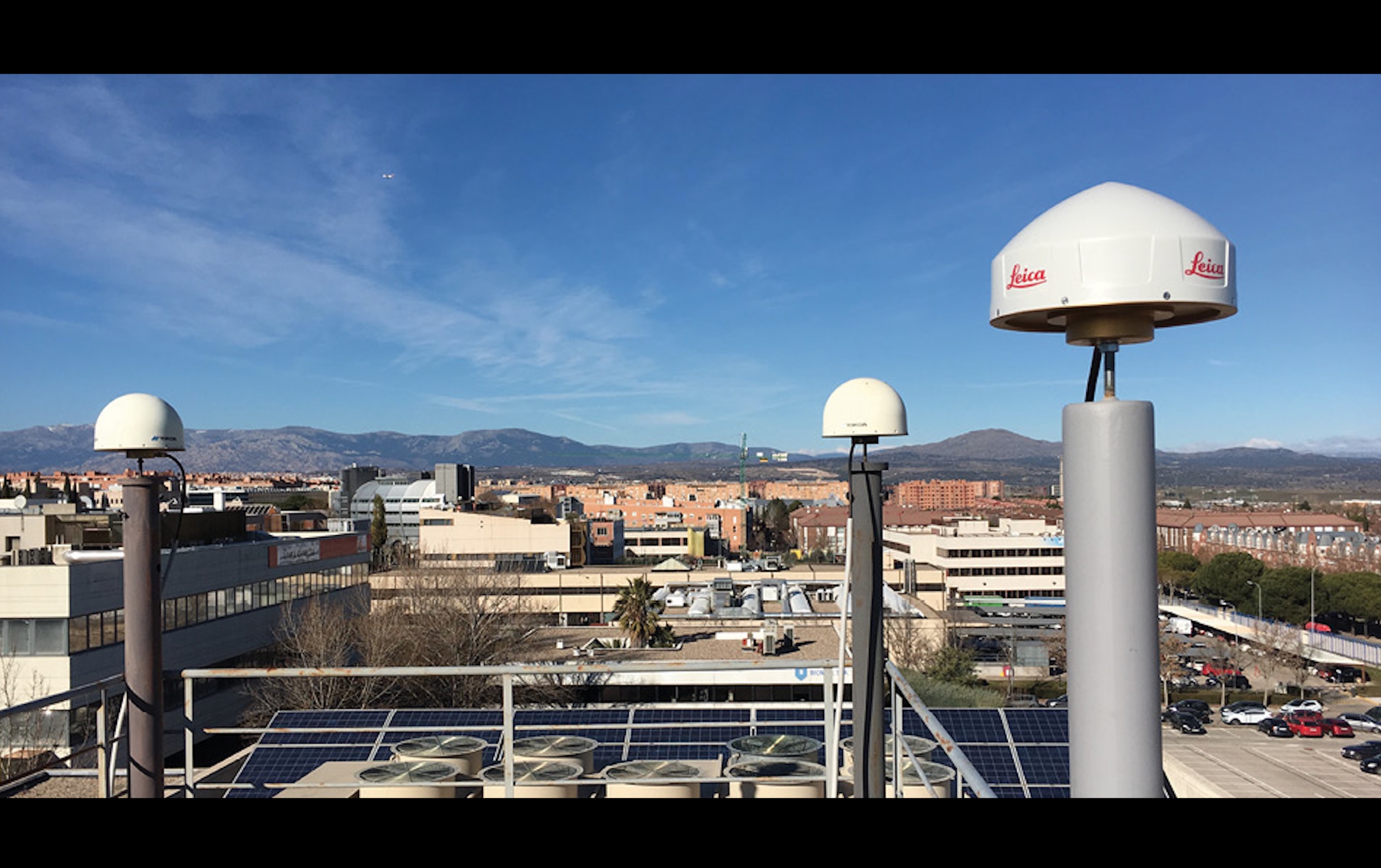
An increasing number of applications require accurate, reliable, and traceable signals for time and synchronization. Key fields of application include banking and finance, telecom networks and electricity grids. GMV’s WANTime is a new time service for the city of Madrid, Spain, distributed using the White-Rabbit network protocol over optical fiber. A pilot customer of the service is currently the Madrid Stock Exchange (Bolsa de Madrid), connected to GMV’s datacenter by a network link of around 50 kilometers.
For redundancy, the service is based on two parallel and independent time generation chains (A and B), each of them driven by a highly stable atomic clock, namely a Passive Hydrogen Maser (PHM). The clocks can be synchronized to UTC by means of GNSS time-transfer to any national timing laboratory. This well-known technique is known as Common-View (CV) and is based on differencing pseudoranges from the same GNSS satellites recorded at the two sites (GMV and the UTC lab). Dual-frequency (DF) pseudorange combinations are normally used in CV to remove ionospheric errors, but single-frequency (SF) CV is also possible.
Clock Synchronization
CV provides the difference between the local clock and the remote UTC time scale. Currently the authors of this article are collaborating with PTB, the Physikalisch-Technische Bundesanstalt in Braunschweig, Germany, to align their clocks to PTB’s realization of UTC, called UTC(PTB). By calculating clock differences over several days it is possible to model and predict the behavior of the clock, and thus to adjust the clock frequency periodically to minimize its deviation from UTC. In our case we adjust our PHMs to UTC using a quadratic model that accounts for the clock phase offset (A0 term, ns), the mean clock frequency offset (A1 term, ns/day), and the frequency drift (A2 term, ns/day2). Every day, we fit the PHM model to the CV results from the 15 previous days, we extrapolate the model to the current day at noon, and we calculate a corresponding frequency correction, that is applied to the PHM by means of a frequency stepper connected at its output. Each PHM is steered independently of the other one.
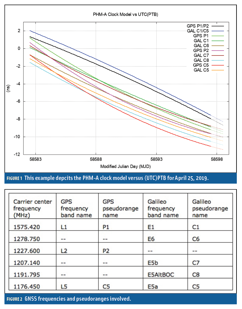
In nominal operations, our CV software uses the well-known iono-free combination of GPS P1 and P2 pseudoranges. In the unlikely event of a problem with this combination, for example due to jamming or interference in the GPS L1 or L2 bands, or even due to a total failure of GPS, we need to have alternative CV methods that ensure the continuity of operations. This is achieved by incorporating Galileo, and also by using SF CV in all the individual GNSS bands. An example of the results is shown in Figure 1 which depicts the PHM-A clock model versus UTC(PTB) for April 25, 2019, i.e., MJD 58598 (Modified Julian Day). The accompanying table (Figure 2) helps to understand the GNSS frequencies and pseudoranges involved. Two DF combinations are used: P1/P2 for GPS (nominal method), and C1/C5 for Galileo. In SF, the iono models used are Klobuchar for GPS, and NeQuick for Galileo.
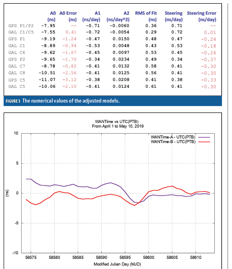
The numerical values of the adjusted models, corresponding to the plots in Figure 1, are shown in the table below (Figure 3). The reference time for the model is T0 = MJD 58597.5. Thus the clock value at any time is calculated as:
A0+ A1* (MJD-T0) + A2* (MJD-T0)2.
“Steering” indicates the frequency correction to be applied to the clock; it is obtained extrapolating the model by one day to MJD 58598.5. In a visual way, the steering is the slope of the tangent to the model curves (Figure 1), evaluated at the extrapolated epoch. The steering is conceived to adjust to zero the instantaneous frequency offset at that epoch. An additional steering correction term is used to adjust the clock phase offset versus UTC to zero in the following 10 days, but this aspect will not be discussed here. “Error” in the A0 term and in the steering is calculated as the difference versus the nominal DF GPS solution (GPS P1/P2). “RMS of Fit” indicates the RMS of the CV data residuals after adjusting the quadratic clock model; the RMS value gives an idea of the uncertainty of the CV method. As can be seen, SF fits are in general nearly twice as noisy as DF ones.
What the Results Indicate
Several facts can be observed from the results. In the first place you can see a relatively large dispersion in the adjusted A0 values, with maximum errors of more than 3 ns versus the nominal solution. This is explained by the combined calibration errors in the two GNSS receivers. The pseudorange delay in each receiver chain can reach a few hundred ns, considering the accumulated effect of the antenna, the antenna cable, and the receiver itself. The total delay can be calibrated with an uncertainty of 2 or 3 ns for each pseudorange signal. Since receiver chain delays are fairly stable, the error in the A0 can be considered constant, and thus it does not affect frequency transfer, but it does affect the time transfer.
The second remarkable fact from the results is that GPS and Galileo provide nearly identical steering results in DF, and that in fact the very small frequency drift of the clock (A2 term) can only be properly estimated in DF. We can observe a large dispersion if the A2 term from the SF solutions, with in fact an opposite sign with respect to DF.
Finally, we can see that the steering error in SF is roughly inversely proportional to the value of the carrier frequency, with smaller values in L1/E1 and larger values in L5/E5a. This makes sense since the ionospheric error in the pseudorange is inversely proportional to the square of the carrier frequency. We can also observe that the minimum steering error in SF is provided by Galileo in E1 (“GAL C1”), which can be explained by the superior performance of the NeQuick iono model as compared to Klobuchar. However the good SF results in L1/E1 must be taken with caution, since this is the signal most likely to be jammed. Interestingly, the E6 signal, unique to Galileo, is the one providing the second-best SF steering, after L1/E1. The worst SF steering is obtained using pseudoranges in the L5/E5 bands, with daily errors of the order of 0.3 ns/day.
Very similar facts are observed from an analogous CV processing of the PHM-B clock. In conclusion, in the worst scenario we would be able to steer the clock to UTC using SF CV in any single GNSS band, with a maximum deviation of 0.3 ns/day, equivalent to 9 ns in one month. This possibility would be very useful in case of persistent jamming or interference in any other band(s), in particular in L1/E1. So far SF steering has not been necessary in WANTime, and the nominal GPS P1/P2 combination has been used since the start of the service provision at the beginning of April 2019. Our deviation from UTC(PTB) so far is shown in (Figure 4).
Manufacturers
At GMV, the PHMs used in this project are model 1008 from Vremya, Russia, distributed in Europe by T4Science, Switzerland. The GNSS receivers are PolaRx5TR from Septentrio, Belgium. The frequency steppers are HROG-10 from SpectraDynamics, Colorado, USA. At PTB, GNSS data used in this experiment has been collected by a GTR55 receiver from MESIT, Czech Republic.
White Rabbit equipment and support is provided by Seven Solutions from Granada, Spain. WANTime is a registered trademark of GMV.
Authors
Ricardo Píriz is an aeronautical engineer by the Polytechnic University of Madrid. He started his career as a Flight Dynamics engineer in the Precise Orbit Determination group at ESOC, the European Space Operations Center in Darmstadt, Germany. Later on he moved to Eutelsat in Paris, as a Mission Analysis engineer in the Satellite Procurement Division. Since 2001 he has been in the GNSS Business Unit of GMV working in several projects, in particular in the GIOVE Mission (the experimental phase of Galileo), and in the Galileo Time Validation Facility (TVF). He is currently Leader of the GNSS Time & Frequency Group.
Pedro Roldán has a Master of Science in Aerospace Engineering from the Technical University of Madrid and in Meteorology and Geophysics from the Complutense University of Madrid. He has worked at GMV since 2013, focused on the definition and development of GNSS and timing algorithms, including algorithms for precise orbit determination, precise point positioning, time transfer, steering of clocks and definition and maintenance of time scales.
Esteban Garbin is an Electronics and Telecommunication engineer who got his Ph.D. from Politecnico di Torino in 2017. His research studies focused mainly on GNSS receivers and signal processing algorithms, particularly for interference and spoofing detection and mitigation. Since June 2017 he has been working for GMV, focusing on different aspects in the GNSS Advanced User Segment solutions division, mainly developing novel concepts on GNSS timing and receivers.


