 BPSK signal magnitude spectrum
The Avionics Engineering Center at Ohio University has developed a real-time, continuously operating GPS Anomalous Event Monitor (GAEM), designed primarily to assist with ground-based and space-based augmentation systems (GBAS and SBAS).
The Avionics Engineering Center at Ohio University has developed a real-time, continuously operating GPS Anomalous Event Monitor (GAEM), designed primarily to assist with ground-based and space-based augmentation systems (GBAS and SBAS).
The GAEM uses high-performance GPS receivers to flag abnormal events originating in the space segment (i.e., satellite anomalies) or the operational environment, such as interference and jamming, multipath, and ionospheric and tropospheric effects.
Upon the detection of erroneous behavior, the monitor records live RF GPS data in the form of intermediate frequency (IF) samples. The RF data are then processed to inspect the spectrum, signal quality, acquisition, and tracking results, together with other aspects that might have an impact on GPS ranging performance.
This article describes the requirements, design, and operation of the GAEM and then presents a series of examples to demonstrate its capabilities.
(To view the many figures and graphs referenced in this article, please download the PDF version using the link, above)
GAEM: The Need and the Benefit
Currently, GAEM hardware is installed at three facilities: the Memphis International Airport in Memphis, Tennessee; the FAA William J. Hughes Technical Center in Atlantic City, New Jersey; and one the Gordon K. Bush Airport of Ohio University, in Albany, Ohio.
The GPS Anomalous Event Monitor is able to perform the following functions:
- operate continuously and automatically, under remote control
- detect and flag a large variety of GPS anomalous events in real-time
- automatically create reports to present all the processing results and to integrate multiple data/information sources that are related to the events
- differentiate causes of the anomalies
- separate anomalies from normal operations
- provide an evaluation of the impact on GPS performance
- provide timely information on detected events and available reports, with a message broadcast to the public or an interested community.
In addition to operators of GBAS and SBAS facilities, these capabilities are useful to specialized users of GPS as well as researchers.
With the RF data and the analysis reports, researchers can investigate any captured events in postprocessing. These postprocessing results not only identify the nature of the event, but also help to determine the origin of it. Furthermore, the consequences of such events can often be directly observed from the reports.
A thorough study on the origin and consequence of past anomalous events is essential for dealing with future anomalies — to predict their occurrence and to minimize the damage. The GAEM also serves as a data archive for those who are interested in evaluating the overall GPS performance at particular locations using historical data.
GPS users can benefit from the estimation of positioning performance in a local environment. Safety-related applications, such as aircraft landing navigation with GBAS and SBAS, have stringent requirements for accuracy, integrity, continuity, and availability.
In general, integrity and accuracy tend to attract more attention, and both can be monitored with the GAEM. Although SBAS already provides certain monitoring functions for GPS integrity, it cannot oversee performance changes in a local operational environment. Users who rely on GPS and SBAS for business purposes need to be able to monitor GPS availability for obvious reasons.
Another example: For GPS positioning in mining and construction operations, a local GPS monitor like the GAEM will be especially helpful. These users demand an extremely accurate positioning capability with a certain level of continuity and availability guarantee for cost reasons.
The GAEM can be most helpful when a sudden change —either positive or negative — occurs in GPS performance occurs.
For example, when new GPS satellites, new frequencies (e.g., L5), or a new signal structure on an existing frequency (e.g., L2C, L1C) are added into the system, they are considered positive changes. The GAEM can monitor and process the new signals with corresponding updates in the RF front-end.
Significant events in a GNSS independent from GPS, such as GLONASS and Galileo, may also have unpredicted effects on GPS. For example, a non-GPS satellite that shares the same spectrum as GPS has the potential of producing in-band interference. Although such interference should be well controlled in principle, a GAEM recording live RF data will definitely help to verify that. On the other hand, the GAEM can also be extended to monitor multiple GNSSs as well as their augmentation systems.
GPS performance at any location depends on the local atmosphere, including troposphere and ionosphere, and the operational environment. Local weather forecasts can predict dramatic tropospheric events, whereas ionospheric effects are often correlated with space weather, for example, the well-known solar activity. Operational environment changes are mostly responsible for local RF interference, multipath, or signal blockage. Data from the GAEM can help to determine whether a local GPS anomaly is due to atmospheric effects or the operational environment.
GAEM Design & Operation
The current architecture of the GAEM consists of three major real-time subsystems — an anomaly detection system, a data collection server, and a remote control, configuration, and monitoring system — with a separate postprocessing network.
The anomaly detection subsystem monitors the status flags and raw measurements output by two commercially available high-quality GPS receivers. If either receiver detects an anomaly, the subsystem generates a trigger.
A few categories of anomalous events are currently being monitored in the system; loss of code lock, loss of phase lock, automatic gain control (AGC) flag, jamming flag, phase distortions, pseudorange steps. The subsystem can also receive triggers from an external source, for example, a local area augmentation (LAAS) ground facility (LGF) or a separate detection box specified by the user.
The data collection server maintains a past history of GPS IF data in a buffer of specified duration, currently 20 seconds in the Ohio set-up. When a trigger is received, the contents of the buffer are written to disk up to a specified end point. The post-trigger duration is currently 5 seconds. Remote clients can access the files generated in this way via the Internet or Intranet, using the tile transfer protocol (FTP) or secure file transfer protocol (SFTP).
The remote control, configuration, and monitoring subsystem (Figure 1) is comprised of file servers, remote console/desktop applications running within the anomaly detectors/GAEM server, an uninterruptible power system (UPS), a power control server, and a camera.
The power server enables independent power-recycling — the capability to switch the power off or on — for each component of the system. This is mainly to enable worst-case recovery, should a component become non-responsive or experience other abnormal behavior.
A webcam enables monitoring of the audio-visual environment of the installed site by authorized clients. The camera surveys physical changes in the environment surrounding the installation that could cause multipath, blockage, or equipment failures. Figure 2 shows the Ohio installation.
The postprocessing network connects one or multiple GAEMs to a super user (a dedicated computer that acts as a remote controller), a few post processing computers, a file server and clients. A diagram of this processing network is shown in Figure 3.
The network can be constructed via Internet or Intranet. The super user acts as the remote controller of the computers and the file server. This user is responsible for managing the file server and sending specific commands to the computers, such as the distributing of computer tasks and software updates. The goal of the postprocessing network is to prepare “quick look” and “detailed look” results that are accessible through printed reports that are generated automatically or a graphical user interface (GUI). Figure 4 shows a step-by-step procedure illustrating how the postprocessing network functions, and Figure 5 shows the cover pages of both quick-look and detailed-look reports.
The quick-look results include overall signal quality measures and system information:
1) system information (location, time of event, antenna type etc.)
2) overall signal quality, approximate CNR (carrier to noise ratio) estimations of all satellites, comparison of visible satellites before and after the trigger sets, signal spectrum
3) output of both reference GPS receivers
4) system log message that reflects the reason and time of trigger, elevation and azimuth angles of the triggering satellite
5) related notice advisories to NAVSTAR users (NANUs), from US Coast Guard <http://www.navcen.uscg.gov/gps/nanu.htm>.
Certain types of events can be easily observed from the quick-look report, such as in-band interference or equipment outage. The detailed-look results come from tracking the visible satellites in the RF data with a research software radio receiver.
The following detailed measurements are available at double precision and a 100 Hz update rate:
1) accurate CNR estimates
2) Doppler and accumulated Doppler
3) carrier phase
4) code-minus-carrier (CMC)
5) navigation data (GPS time decoded from the signal, etc.)
All of these measurements are independently observed and collected using two software receivers; one receiver uses block processing techniques and the other simulates receiver tracking loops. A user can cross-compare different satellites and find out what could have been wrong with the target satellite.
The block processing receiver is robust and resistant to signal interruptions, which is an ideal choice for anomaly analysis. The software tracking loops provide high-rate receiver measurements, which are especially useful because regular GPS receivers often temporarily lose their outputs during an anomaly.
Application Examples: Anomalies or Normal Operations?
When a change in GPS performance or signal is detected, the first thing to determine is whether an anomaly is causing the change or that it just reflects a result of normal operations. A normal operation can be scheduled maintenance, in which case it can be verified with GPS authorities, or it can be a normal reaction by satellites to certain incidents.
The nature and origin of a normal operation that affects GPS performance needs to be determined in order to avoid false alarms, because regular GPS receivers may not anticipate them. As an advanced feature, the GAEM will be able to predict the duration of such events and consequently forecast any future changes related to it.
On the other hand, if the detected change does not stem from a normal operation, it should be considered an anomalous event. Such events can happen in the space segment or in the user segment, that is, they may arise in the satellites, from the signal propagation path, or from the local environment.
The following discussion shows a few examples of the GAEM handling both normal operations and anomalous events. The postprocessing results shown in this section are all included in the reports that the GAEM automatically generated for each of the events.
Satellite Maintenance
Scheduled and predicted satellite maintenance shouldn’t be included in the anomaly category. However, the GPS receivers will detect off-nominal behavior in the signal because of it. Without external information, the anomaly detection system would be triggered and record this event. However, the GAEM is able differentiate an expected maintenance by retrieving information from the websites of GPS authority.
On Aug. 17, 2007, the GAEM detected an event on a GPS satellite, space vehicle number (SVN) 52/PRN31. The system log message shows that at GPS time 224741.0 both reference receivers simultaneously lost lock on the satellite’s signal. As part of the quick-look report, the outputs of both receivers recorded for one hour can be found in Figure 6. The graphs on the left represent data derived from the output of Receiver 1, while the graphs on the right side of the figure represent data from Receiver 2.
Viewed from top to bottom, the graphs show sequentially differenced pseudorange measurements, sequentially differenced carrier phase measurements, code-minus-carrier measurements, carrier-to-noise ratio (C/N0), and receiver lock time, respectively.
All the measurements from both receivers appeared to be normal, until the moment both receivers lost lock. The quick-look report also showed that the signal strength appeared to be regular, and spectrum data reveals no noticeable interference.
Even though the GPS receivers didn’t continue to track this satellite, a 25-second long RF data file was recorded and processed with the software radio receiver. Acquisition and tracking measurements from the software radio receiver also seemed normal, except that the health bits in navigation data were all set to one, which indicate that the satellite should not be used, according to the Interface Control Document GPS-200 (ICD-GPS-200).
A NANU message related to this event, citing the satellite’s pseudorandom noise (PRN) number and time, is also included in the quick-look report:
NANU TYPE: FCSTSUMM
NANU NUMBER: 2007090
NANU DTG: 142132Z AUG 2007
REFERENCE NANU: 2007086
REF NANU DTG: 101333Z AUG 2007
SVN: 52
PRN: 31
START JDAY: 226
START TIME ZULU: 1424
START CALENDAR DATE: 14 AUG 2007
STOP JDAY: 226
STOP TIME ZULU: 2130
STOP CALENDAR DATE: 14 AUG 2007
2. CONDITION: GPS SATELLITE SVN52 (PRN31) WAS UNUSABLE ON JDAY 226
(14 AUG 2007) BEGINNING 1424 ZULU UNTIL JDAY 226 (14 AUG 2007)
ENDING 2130 ZULU.
The NANU message matches the health bits, and it becomes obvious that the loss of lock was due to scheduled maintenance.
Although this example may seem trivial since both the GPS NANU and health bits can clearly identify the cause of the event, such an event can prove more interesting if, for instance, the GPS NANU and health bits are not synchronized.
On April 10, 2007, a satellite maintenance issue arose on SVN54/PRN 18. A Federal Aviation Administration (FAA) report of the event, referenced in the Additional Resources section at the end of this article, indicates that a NANU message forecast scheduled maintenance of this satellite some time between 13:30 GMT on April 10 and 1:30 GMT on April 11.
The actual maintenance work initialized at approximately 15:53 GMT on April 10, while the satellite health bit was still set to “healthy,” apparently by mistake. Large range errors occurred before the health bit was corrected at 17:04 GMT. Having RF data, GPS receiver output, and the NANU all included in one report would have greatly helped users to understand what had happened.
Non-Standard Code
Although seemingly “abnormal,” the second example here is not an anomaly either. As documented in ICD-GPS-200, in order to protect users from receiving and utilizing erroneous satellite signals, GPS satellites switch off regular broadcast of C/A code and P/Y code and transmit the non-standard C/A code (NSC) and non-standard Y code (NSY) in case of “unhealthy” conditions on the spacecraft.
For example, non-standard code will be received when a malfunction occurs in the satellite reference frequency generation system, a certain data failure in satellite memory, or scheduled maintenance. Therefore, the transmission of non-standard code is considered a normal operation in itself, even though it may reflect a glitch in the satellite.
The NSC consists of alternating 0s and 1s transmitted at the C/A code chipping rate, which is designed to have negligible effect on tracking other healthy GPS satellites. In many cases over the years, however, the transmission of NSC could not be predicted, and it caused an unexpected change in the performance of user equipment. So, in effect, such an anomaly affects GPS availability and integrity.
Multiple events have been observed, and as an example, we will analyze the one recorded on November 28, 2006 at 12:38 p.m. EST, when SVN38/PRN 8 was switched to NSC mode.
Figure 7 displays a screen shot of the GAEM GUI that demonstrates quick-look outputs from this event. The upper left graph illustrates estimated CNR as a function of time for 26 seconds for all visible 32 PRNs. In that graph, red corresponds to strong satellites and deep blue corresponds to unavailable satellites. A red vertical line is used to indicate the approximate time of the trigger.
The two graphs located on the lower left-hand corner of Figure 7 show the average signal strength of all 32 PRNs before the trigger and after the trigger, which is used to identify change of available satellites due to the possible anomaly. The upper graph on the right illustrates the signal spectrum in a blue line, estimated using one millisecond of signal at the end of the data. For reference and comparison, the red line in this graph represents the signal spectrum averaged over 100 milliseconds at the beginning of the data before the system was triggered.
The middle right-hand graph provides a three-dimensional time-frequency plot showing the change of signal spectrum over time, and the lower right graph is a top view of that same time-frequency plot.
Figure 8 is a screen shot of the GUI displaying the detailed-look process, which shows the tracking results for PRN8. The upper, middle, and lower graphs on the left correspond to graphs of the C/N0, accumulated Doppler, and the differential of integrated Doppler measurements, respectively. The graphs on the right show the carrier phase tracking residual, code phase tracking residual in form of code minus carrier and navigation data bits, respectively.
If the data bits have been decoded correctly, the GPS time of the beginning of the observation window is also shown. In the detailed-look process GUI as shown in Figure 9, a user can simultaneously zoom in on the same part of the run-time in all graphs. The quick-look and detailed-look results presented in the GUIs are contained in the corresponding printed postprocessing reports.
As can be seen from Figure 7, the C/N0 estimation of PRN 8 shows loss of signal around the 19th second into the file. Figure 8 shows that the tracking of PRN 8 seems to be in a normal mode up until the moment when it becomes absent.
A zoomed-in view around the 19th second is shown in Figure 9 and provides more signal-tracking details. More interestingly, the GPS time was decoded from all the navigation data bits recorded before the loss of PRN 8, from which the occurrence of this event can be precisely synchronized to GPS time.
The signal spectrum and time-frequency plot in Figure 7 contain irregular components that are not standard in a regular GPS signal spectrum. Two spikes are located at approximately 500 kHz and -500 kHz at a sustained level for six seconds until the end of the observation window.
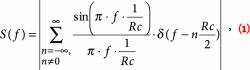
Recall that the NSC is a BPSK (Binary Phase Shift Keying) signal with alternating 0s and 1s at a chipping rate of Rc = 1.023 Mbps. This signal has a magnitude spectrum given by the formula found at the top of this article (above, right), which consists of a series of impulses under the envelope of a sinc wave with a two-MHz null-to-null bandwidth. Within the two-MHz bandwidth, two major impulses are located at +/- Rc/2, which are responsible for the signal spectrum observed in Figure 7. A further study shows that during the six-second outage, NSC can be acquired and tracked in the recorded RF data. As a result, we can differentiate non-standard code broadcasts from truly anomalous GPS outages.
Ionospheric Effects
The effect of the ionosphere on GPS signal transmission has received considerable attention ever since the early days of the Global Positioning System. Monitoring ionospheric effects such as scintillation serves to ensure the integrity of safety-of-life systems as well as everyday users.
Since the GAEM system started continuous operation, hundreds of events have been collected at the Ohio installation alone. We believe that a significant number of events collected in late 2006 could be attributed to ionospheric effects.
The year 2006 is not supposed to be a peak year for sunspot activity according to the 11-year solar cycle. However, on most of the days from November 30 to December 17, 2006, sunspot activities were reported with magnetic classes of BG, BD or BGD, while the sunspot activities at a normal day is usually labeled as Class A or B. (For a discussion of the U.S. Air Force and National Oceanic and Atmospheric Administration classifications, see the reference in Additional Resources.) The sunspot activities identified as BG, BD, or BGD are considered potentially problematic for radio transmission.
Figure 10 shows a screen shot of the quick-look output GUI for an event collected on December 6, 2006, at 12:56 p.m. EST. Apparently PRNs 4, 8, 11, 17, and 28 could be acquired. Only PRN 11, however, can be considered a strong signal, and the power level of PRN 4 would make it difficult to track.
Fortunately, the GAEM block-processing software receiver does not easily lose lock, and the tracking results of PRN 4 are demonstrated in Figure 11. The CNR measurement fluctuates around 33 dB-Hz and can be as low as 30 dB-Hz. Such effects are sometimes referred to as amplitude scintillations.
Having a total of five visible satellites with only one strong signal can result in degraded positioning accuracy as well as system integrity. Furthermore, because the CNR of a GPS signal largely depends on individual antenna patterns. Some antennas could receive fewer than four satellites in this situation. When that happens, ionospheric effects also affect the continuity and availability of GPS and SBAS positioning. (At the time this data was collected, GAEM used a choke ring antenna. Now it connects to a pinwheel + multipath limiting antenna or MLA.)
The GAEM is able to associate the observed the results with space weather information and determine the cause of such events. More importantly, knowing the cause, it can forecast the occurrence of the same type of events.
Multipath
Our final example deals with the solution of an obscure problem involving a series of events observed on a single satellite.
The Ohio GAEM system was installed on the Ohio University campus before it was moved into the OU airport in 2008. From June to September 2007, 14 events were recorded for PRN 21. Although no NANU message related to these events could be located, both reference GPS receivers reported loss of lock during all of the events. However, receiver outputs did not contain enough information to explain why loss of lock happened at these particular moments.
The software radio receiver can provide high resolution and update rate of signal tracking results. CNR measured with the software receiver during one of these events is shown in Figure 12, in the upper left figure. It carries a clear sinusoidal variation with a peak-to-peak magnitude of approximately two decibels.
Code-minus-carrier (CMC) calculations are also a helpful diagnostic measurement. In the GPS receivers used in GAEM, code phase is measured using pulse aperture correlators and filtered by loop filters and carrier smoothing. The approach has minimized the effects of error sources such as multipath but is less effective as an error indicator.
The code phase measured with the software radio receiver uses standard correlator spacing and is unfiltered. Although these raw measurements contain much more noise, they can help in analyzing error sources.
In the middle right graph of Figure 12, the CMC also displays a sinusoidal pattern at the same oscillatory frequency as CNR. The appearance of this pattern in both CMC and CNR suggests the possibility of multipath in the signal, which could not have been recognized otherwise.
Although this initial investigation indicated the nature of the anomalies, their exact cause remained unknown. However, the phenomena were found to be geometry-dependent. The satellite azimuth and elevation angles recorded in the system log message for each of the events are reflected in the azimuth-elevation plot in Figure 13.
The azimuth angles measured in 11 events were concentrated within the range of 170 to 200 degrees, while the remaining three had an azimuth of approximately 310 degrees. The elevation angles, on the contrary, spread out in the range of 35 to 80 degrees. Notice that the mask elevation angle of the receivers had to be set to 35 degrees in a suspected multipath environment.
The consistency of azimuth angle measurements further supports the assumption of multipath. These measurements also make it possible to identify the source of multipath.
Figure 14 contains an aerial photo that provides a bird’s eye view of the antenna and surrounding environment. The red circle marks the building where the antenna is installed. To the southeast of this building is a white dome, seen in the lower right-hand corner, which is the Ohio University convocational center. The curved roof of the convocational center forms many reflecting surfaces at various attitudes.
Because of the roof’s curved surface, signals from a wide range of elevation angles and a smaller range of azimuth angles can be reflected off of it and received by the antenna. The red arrows illustrate a possible path for the signal reflection, which comes from a satellite with the azimuth angle of approximately 170 degrees. As further indication that the convocational center dome was the culprit, these multipath events no longer occurred after the Ohio GAEM installation moved to the OU airport, shown in Figure 2.
What’s the Plan?
The GAEM has been further developed to enable it to process SBAS signals. In the future, this system will also be able to monitor other GNSS signals, including the following functions:
1) intelligent analysis: enable the GAEM to act like an analyst and give a definitive answer
2) customized monitoring: capture events that would affect a user-specified performance property
3) additional data sources: troposphere status from local weather input, ionosphere status for space weather input, and multipath environment from on site camera
4) networking multiple locations: to easily identify whether an event occurred in a local area or can be attributed to the space segment
5) wide band data collection: increase the monitoring bandwidth from 2.2 MHz to 24 MHz, the full GPS bandwidth, at L1, L2, and L5 frequencies
6) hardware acceleration of the postprocessing: data samples using a field-programmable gate array (FPGA) to greatly reduce the calculation time..
Acknowledgements
This research was supported by the Federal Aviation Administration Aviation Research Cooperative Agreement 98-G-002.
Additional Resources
Doherty, P. and S. H. Delay, C. E. Valladares, and J. A. Klobuchar, “Ionospheric Scintillation Effects in Equatorial and Auroral Regions,” Proceedings of ION GPS 2000, Salt Lake City, Utah, p. 662-671, September 2000
Federal Aviation Administration, “Global Positioning System (GPS) Standard Positioning Service (SPS) Performance Analysis Report #58,” July 31, 2007
GPS JPO (Joint Program Office), ICD-GPS-200 (GPS Interface Control Document), prepared by ARINC Research, April 2000
USAF (U.S. Air Force) and NOAA (National Oceanic and Atmospheric Administration), Sunspot data, available: <http://solarscience.msfc.nasa.gov/greenwch.shtml>
Zhu, Z., and S. Gunawardena, M. Uijt de Haag and F. van Graas, “ Advanced GPS Performance Monitor,” Proceedings of ION GNSS 2007, Forth Worth, Texas, September 2007
Zhu, Z., and S. Gunawardena, M. Uijt de Haag and F. van Graas, “Satellite Anomaly and Interference Detection Using the GPS Anomalous Event Monitor,” Proceedings of ION 63rd Annual Meeting, Cambridge, Massachusetts, April 2007


