
A look at algorithms developed for the real-time detection and localization of GNSS interference sources, and an investigation into last year’s disruption at Dallas-Fort Worth International Airport.
ZIXI LIU, SHERMAN LO, TODD WALTER, JUAN BLANCH, STANFORD UNIVERSITY
GNSS serves several safety-of-life applications in aviation such as precise navigation for landing operations, collision avoidance and Air Traffic Control (ATC). GNSS interference events happening near airports can severely affect safe operations in the airspace and can be hazardous for aircraft on approach or landing. Many interference events occur throughout the year, affecting U.S. air traffic. A notable interference event happened at Dallas-Fort Worth International Airport (KDFW) in October 2022, causing widespread disruption. This incident resulted in multiple aircraft reporting GPS unreliable within 40NM of the airport, closure of a runway and rerouting of air traffic.
The growing dependence of critical and safety-of-life systems on GNSS makes the ability to rapidly detect and accurately localize the presence of GNSS interference events increasingly
important. In this study, we designed a system of algorithms that can monitor a given airspace for potential GPS interference events and can search for the most likely location and power level of the source if an interference event is detected. The goal is to have this algorithm quickly identify and find the interference threat and enable physical removal of the jamming source.
Our algorithms have been tested using recorded ADS-B transmissions from known interference events. The testing results demonstrated the ability to detect a static omnidirectional interference source within a few minutes of the onset of transmission and identify the location of the interference source within a small region in which enforcement could be directed. The source of the GPS disruption that affected the Dallas airport has still not been identified. Therefore, in this study, we also performed a detailed investigation on that event and applied our algorithms to help provide an estimation and characterization of the potential jamming source.
Automatic Dependent Surveillance—Broadcast (ADS-B)
Automatic Dependent Surveillance—Broadcast (ADS-B) is a surveillance system on aircraft that broadcasts the GNSS derived position every 0.4 to 0.6 seconds on a 1090 MHz frequency band (DO-260B RTCA [1]. The benefit of using ADS-B data for interference detection and localization, compared with traditional methods such as radio direction finding, is that it’s less time consuming. In addition, this crowd-sourced data from multiple aircraft offers broader coverage of the impacted airspace. The drawback to this method is ADS-B messages do not contain information from the GNSS receiver, such as carrier to noise ratio (C/N0), that indicates jamming. However, ADS-B messages have some built-in parameters that indicate the integrity and accuracy levels of the reported GNSS measurements.
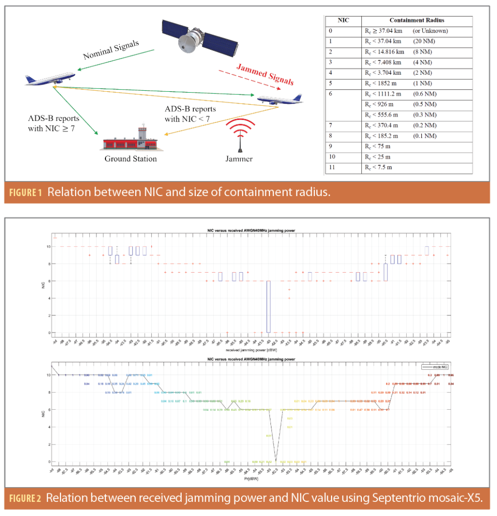
In our research, we use the broadcast Navigation Integrity Category (NIC) to estimate the quality of GNSS reception. NIC describes the size of an integrity containment radius that the current horizontal position is guaranteed to be within, with 99.999% probability. Figure 1 shows the tables for NIC and how it reacts under different circumstances [2]. According to ADS-B equipment performance requirements defined in Title 14 of the Code of Federal Regulations, under normal circumstances, the aircraft’s NIC value must be ≥ 7 (containment radius less than 0.2 nautical miles). When NIC equals to 0, the corresponding errors are much worse than typical GNSS performance. When GNSS performs this poorly, unless there’s an incorrect setting of the ADS-B system, it’s likely the aircraft has been severely affected by a jammer.
Approaches
The goal of our research is to design a system of algorithms that can monitor any given airspace for potential GPS interference events. The algorithms can provide immediate detection of the interference threat and reliable information about the most likely location of the interference source.
Step 1: Detecting the interference event.
We developed a Bayesian updating based algorithm that can provide rapid detection of interference threats. It starts with a prior probability of whether an area contains GPS jamming and updates the probability using measurements collected within each 30-second time window, assuming during each time window we observed m new ADS-B data points. Within those m points there are n flights and each flight has m(k) points. And we split the ground map under the given airspace into small grids. Then the probability of jth grid containing interference can be estimated using:
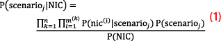
Where NIC ∈ is a vector of all NIC values from the m measurements. Ρ(scenarioj) is the prior probability of jth grid containing interference. This can be calculated using historical data collected from that grid. It helps account for the fact that different areas have different likelihoods of containing GPS interference. For instance, jamming and spoofing occur regularly in the Eastern Mediterranean but rarely within U.S. domestic airspace. Ρ(NIC) is the probability of current NIC values being measured. This can be used to adjust for measurement noise such as aircraft performing high dynamic maneuvers might report low NIC values even without interference.
is the probability of current measured NIC values being seen under the condition of assuming the current grid contains interference. This is calculated by comparing the differences between the measured NIC versus expected NIC. The final step is to normalize probability among all grids, including the imaginary grid that represents the scenario of no interference, such that the probabilities from all scenarios can be summed into 1. If the no-interference grid has the highest probability, then there is no interference in current airspace. Otherwise, if any other grids have higher probability, there is interference in current airspace.
Step 2: Localizing the interference source.
Once the event is detected, the quality indicator from ADS-B data can be used to estimate the most likely location and power level of the interference source. We implemented an optimization algorithm that minimizes the difference between estimated received jamming power and the measured received jamming power
at each aircraft reported position point. The algorithm starts with an initial assumed location and power level of the interference source, then applies Gauss Newton method to search for the minimum point.
Received Jamming Power from NIC
Because ADS-B data does not provide direct information about GNSS reception and received jamming signals, we need to first estimate the relation between NIC and the amount of received jamming power. We developed a prototype empirical mapping by running experiments on different GPS receivers when subjected to different types of jamming [3]. Figure 2 shows a sampled plot of the experiment results. The x-axis is the received jamming power at the aircraft antenna and the y-axis is the NIC value. For each power level, we measure the protection level of the position and convert it into NIC value based on the table shown in Figure 1. The results give us an observable relation between the received jamming power and NIC value. The top plot shows the box plot of the experiment result. The bottom plot shows the percentages of points that were at corresponding NIC value. The mode value at each power level is connected by a black line. This experiment helped us understand the expected amount of received jamming power for a given NIC value and the corresponding variances.
Gauss-Newton Method
Each measurement contains the location of the aircraft (xa, ya, za) and the received jamming power measured based on NIC value (Pra). Given an assumed jammer location (xj, yj, zj) and transmitted power level (Pt), we can predict or estimate the amount of jamming power received at each aircraft using the Friis formula [4]:

Where Pr is the received power in watts, Pt is the transmitted power in watts, λ is the transmitted signal wavelength in meters, d is the distance between transmitter and receiver in meters, and Gt Gr are the transmit and receive antenna gain.
The objective function is to minimize the difference between the measured and predicted received jamming power:

Where W is the weight matrix that allows us to design the mechanisms behind the model based on the known information about dataset collected from different airspaces. The weight matrix can be thought of as inversely related to the measurement’s covariance matrix. The diagonal elements represent the variance of received jamming power at the given NIC value. The off-diagonal elements model the time correlation between data points collected from the same airplane.
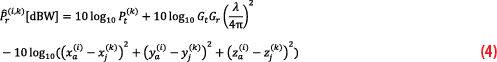
To solve the least square problem, we need to first convert the power unit from Watts to dBW to avoid numerical error caused by small power values. The received jamming power at ith aircraft location and kth designed jammer location is:
Then we need to linearize the objective function near the local state at each iteration using first order approximation. At kth iteration:
The final step is to apply the Gauss Newton method to update the design state X until converged:

Results and Analysis
Validation with known interference event
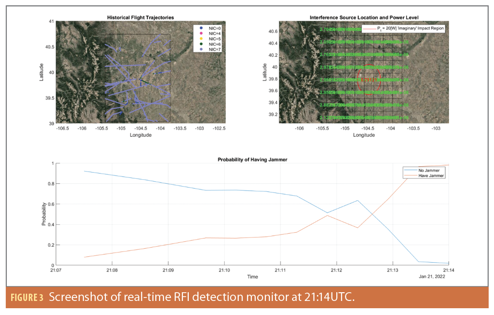
In this article, we validated and tested the algorithm on a GPS interference event that happened near Denver International Airport (KDEN) in January 2022. Figure 3 shows the detection of interference through monitoring the probability of whether the area contains GPS jamming using ADS-B data collected from every 30-second time window. The upper left plot shows ADS-B data observed from the 21:07 UTC to 21:14 UTC color coded in terms of NIC values. The bottom plot shows the variation of the probability in current airspace with respect to time. The red line is the probability of having a jammer in current airspace and the blue line is the probability of not having a jammer. The algorithm starts with a prior probability of 10% (red line) at 21:07 UTC. The overall probability of having an interference source increases as time passes, and it reaches 95% at 21:14 UTC. The upper right plot shows the probability of each scenario at 21:14 UTC. The grid with the highest probability is the most likely space that contains interference. During the event, the earliest pilot reports (PIREPS) on GNSS issues were received at 22:25, but we are able to identify the existence of an interference event at 21:15, which is about an hour before. By looking at the ADS-B data we collected, the first NIC=0 data point appeared at 20:58. If we use that as the time when the jammer started transmission, our algorithm was able to identify the existence of jamming within less than 20 minutes and more than an hour before ATC was made aware by the PIREPS.
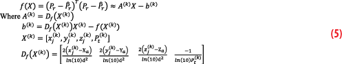
Once the event has been detected, the algorithms then search for the local minimum of the residuals using data collected from the past 2.5 hours. Figure 4 shows the result obtained by running the Gauss Newton method for 15 iterations. The plot on the left shows the variation of the estimated jammer location at each iteration. The arrow indicates the movement direction of each iteration. The blue circle is the starting point or the initial assumed jammer location. The dark pink circle is the final location at the 15th iteration. The plot on the right shows how residuals and transmitted jamming power varies for each iteration. The result shows clear convergence.
Application on recent unknown interference event
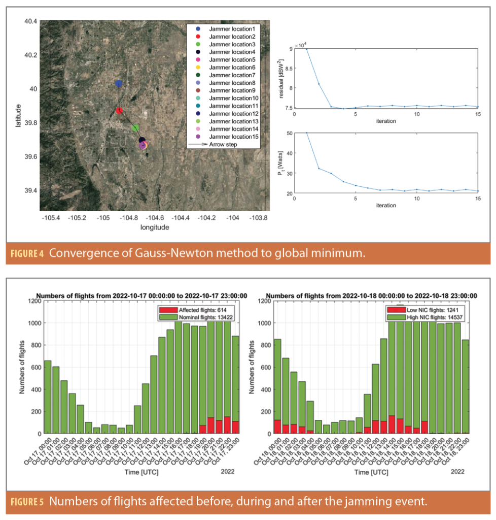
Now that we have the algorithms designed and tested, it is time to apply it to the more challenging interference event that happened near Dallas airport in October 2022. This event caused dramatic impact and widespread disruption. The cause or the source of the interference is still unknown today; we did our own investigation and have run our algorithm to estimate the most likely jammer location with a probability heatmap. After removing some anomalies that contain misleading information, we obtained a better understanding of the overall jamming situation about the Dallas event [5]. Figure 5 shows the timeline using a histogram of the numbers of flights that have been affected. The significant impact of the jamming started at around 10/17/2022 19:21:00UTC and ended at around 10/18/2022 19:10:00UTC. The event lasted about 24 hours with a 5-hour gap in between when no aircraft appeared to be affected.
Figure 6 shows how airplanes have been affected spatially. The impact region stays roughly the same before 10/18/15:00UTC. The shape of the region with low NIC values forms a cone that is aiming toward 30°or 210° azimuthally. This direction does not align with any runway at Dallas airport or any nearby highways. It is possible the interference source is being broadcast by a directional antenna or that it is omnidirectional, but the jamming signal has been blocked from the east and west side by nearby obstructions. During 15:00UTC to 16:00UTC, the impact region gradually moved to the southeast of the airport. This change happened near the end of the event and indicates the jammer might also be non-static in terms of power level, direction and/or location.
Now that we have a better view of the overall jamming situation, we can apply our localization algorithm with an assumption that the interference source is static with a directional antenna. The direction can be tuned by changing the antenna gain of the transmitter (G_t) in the Friis formula. In addition, data collected after 10/18/15:00UTC was ignored because the non-static behavior of the jamming that happened near the end of the event is difficult to characterize.
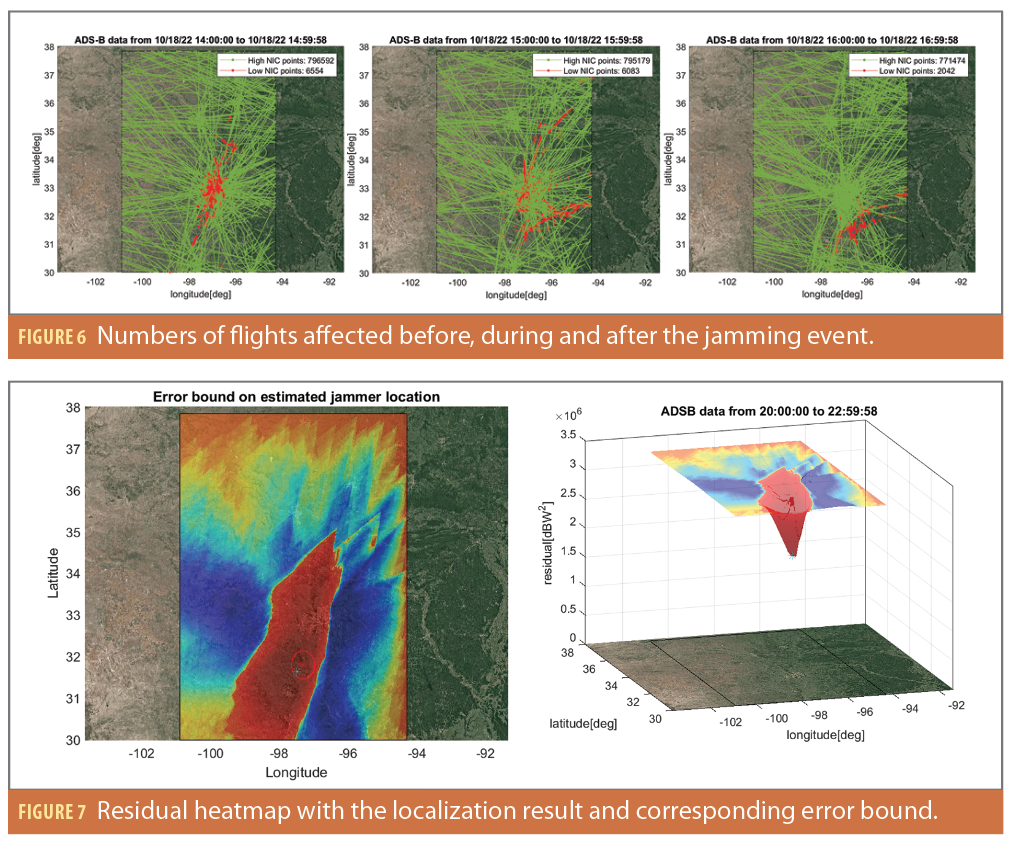
Figure 7 shows the heatmap of the objective function at each possible jammer location. Red indicates smaller residuals and therefore higher probability of being the true jammer location. The objective function also estimates the power level of the interference source. Therefore, to visualize the objective function in 3D, at each possible jammer location, only the most likely transmitted jamming power is used to calculate the corresponding residuals. The cyan star shows the global minimum point on the residual plot. The red circle and its center point together show the final estimated jammer location with an error bound. This is obtained by running the Gauss Newton method on an initial assumed jammer location for multiple iterations until converged. The heatmap shows the objective function points strongly toward a global minimum point. The optimization result has a small error bound. This means the assumption of directional antenna fits the current dataset. The localization result indicates the most likely location of the jammer is to the southwest of the airport near Waco. However, as the source is currently unknown, the accuracy of the prediction cannot be confirmed.
Conclusion
We designed a system of algorithms that can identify the presence of interference within 15 minutes of the first observation of transmission. In addition, it can identify the most likely location of the source of interference within a small degree of error. The algorithms also provide additional uncertainty and confidence information on the localization result by calculating the error bound and generating a probability heatmap.
We applied our algorithms to a recent interference event near Dallas airport. The source of disruption has still not been identified, but our resulting information shows the potential source could have been using a directional antenna with a non-static power level. We also provided a clearer view of the Dallas event in terms of timeline and impact region. We hope our investigation results can help further identify and characterize the properties of the interference source.
Acknowledgements
The authors thank the Federal Aviation Administration (FAA) for sponsoring this research. The authors also thank the OpenSky Network [5] and ADS-B Exchange for providing ADS-B data for this study.
This article is based on material presented in a technical paper at ION GNSS+ 2022, available at ion.org/publications/order-publications.cfm.
References
(1) DO-260B RTCA (Firm) (2011). Minimum Operational Performance Standards (MOPS) for 1090 MHz Extended Squitter Automatic Dependent Surveillance-Broadcast (ADS-B) and Traffic Information Services-Broadcast (TIS-B). RTCA, Washington, DC,
USA.
(2) Office of the Federal Register, National Archives and Records Administration (2013). 14 CFR § 91.227 – Automatic Dependent Surveillance-Broadcast (ADS-B) Out equipment performance requirements. [Government].
(3) Chen, Y.-H., Liu, Z., Blanch, J., Lo, S., and Walter, T. (2023). A RFI testbed for examining GNSS integrity in the various environments. In Proceedings of the 2023 International Technical Meeting of The Institute of Navigation, pages 1032–1042.
(4) H. T. Friis (1946). A note on a simple transmission formula. Proceedings of the IRE, 34(5):254–256.
(5) Liu, Z., Blanch, J., Lo, S., and Walter, T. (2023). Investigation of GPS interference events with refinement on the localization algorithm. In Proceedings of the 2023 International Technical Meeting of The Institute of Navigation, pages 327–338.
(6) Schäfer, M., Strohmeier, M., Lenders, V., Martinovic, I., and Wilhelm, M. (April 2014). Bringing up OpenSky: A large-scale ADS-B sensor network for research. In ACM/IEEE International Conference on Information Processing in Sensor Networks.
Authors
Zixi Liu is a Ph.D. candidate at the GPS Laboratory at Stanford University. She received her B.Sc. degree from Purdue University in 2018 and her M. Sc. degree from Stanford University in 2020.
Sherman Lo is a senior research engineer at the GPS laboratory at Stanford University.
Todd Walter is a Professor of Research and director of the GPS laboratory at Stanford University.
Juan Blanch is a senior research engineer at the GPS laboratory at Stanford University.

