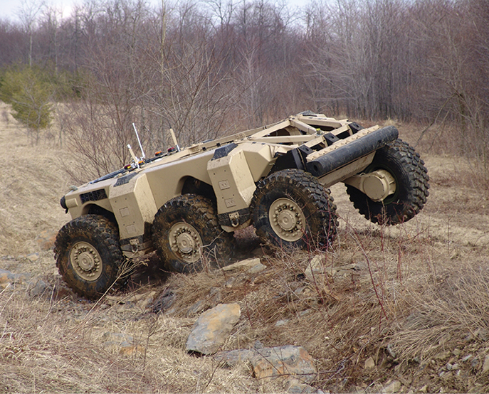
The addition of alternative sensors such as cameras, magnetometers, and small ranging radios increases the likelihood of a mismodeled and/or faulty sensor, affecting the accuracy and performance of the overall navigation solution. Unlike two-sensor systems such as GPS-inertial integration, systems of three or more sensors present the problem of ambiguity as to which sensor is adversely affecting the solution. This presents the need for a robust framework that can maintain navigation integrity despite the additional sensor modalities.
Much time and effort has been invested into alternative navigation to operate independently of GNSS using sensors such as vision-aided navigation, navigation by very low-frequency radio, and more recently, through map-matching of magnetic anomalies. The primary reason behind these efforts is the need for navigation when GNSS signals are unavailable due to occasional outages, signal obscuration or in contested environments due to jamming or spoofing. The increased possibility of GNSS outages brings the need for error characterization and integration of a multitude of alternative sensors into a single platform with a robust integrity framework. The integrity framework must be capable of monitoring all sensor measurements to perform fault detection and exclusion (FDE) of sensors experiencing adverse mismodeled effects. Additionally, the framework must be able to solve for and apply corrections to the stochastic model to account for these effects.
There has been extensive research into integrating two sensors on the same platform and assessing sensor measurements. However, when more than two sensors are incorporated on the same platform, identifying the culprit sensor becomes challenging. One method of handling sensor faults is through solution separation, using a main filter and several subfilters, each excluding one sensor. However, this is not as effective in detecting faults that do not result in a significant difference in state estimation between the uncorrupted and remaining (corrupted) subfilters. Faults producing such differences resulted in undetected faults when compared with an FDE with a more rigorous statistical algorithm
A new algorithm, Sensor-Agnostic All-Source Residual Monitoring (SAARM), uses a sum of squared residual covariance Mahalanobis distances as a moving average χ2-test. Such a technique is part of a larger framework known as Autonomous and Resilient Management of All-Source Sensors (ARMAS).
Background
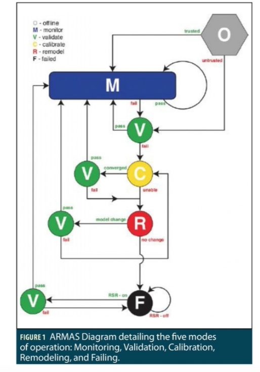
The ARMAS framework draws from several research papers and includes such concepts as FDE, re-calibration, and remodeling of faulty sensors and combines them into one robust framework. The ARMAS framework collects input measurements from each sensor and categorizes them into five major modes of operation: monitoring, validation, calibration, remodeling, and failing. Figure 1 displays the modes of operation. Of these five modes, only the sensors in monitoring mode are able to affect the navigation solution. The remaining modes allow the sensors to be re-calibrated and/or remodeled so that they can be validated and reused in the navigation solution. Sensors that have been placed into failure mode are allowed to be recovered via a process known as Resilient Sensor Recovery (RSR), whereby the sensor may re-attempt validation after a user-specified time period and potentially be placed back into monitoring mode.
The SAARM algorithm considers sensors operating in monitoring mode, and in the event of a fault, determines which sensor should be excluded for possible re-calibration and/or remodeling. SAARM employs multiple filters and calculates the Mahalanobis distances for each sensor/subfilter pair. The framework leverages past research of modeling and stochastic error estimation for one- and two- sensor systems to derive an overarching heterogeneous sensor-independent algorithm. This algorithm seeks to, first, evaluate if there is a potential inconsistency in the navigation solution and second, to isolate and exclude the sensor causing such inconsistency for follow-on validation, calibration, and/or remodeling. SAARM operates within the ARMAS framework which allows additional modeling and stochastic error estimation techniques to be added and evaluated in parallel, depending upon the application. As such, the approach is a scalable, modular framework that can be added or modified as sensors are added or removed from a system, or as the modeling of particular sensors matures.
This article focuses on sensors that are in monitoring mode and are directly affecting the navigation solution. The monitoring mode contains the FDE layer that uses the SAARM algorithm to determine if there is a fault in the navigation solution, and to determine which sensor is the culprit causing the fault. Once the culprit sensor is determined, the sensor is removed from the monitoring mode and placed into validation mode at which time the sensor can no longer affect the navigation solution. The ARMAS/SAARM framework presents the navigation solution to the user as a single Bayesian filter that is supplied by all measurements vetted by this FDE subfilter. Previouysly, the SAARM algorithm had been tested with only synthesized data and compared with conventional filtering techniques. This article incorporates real-world measurement data in a 3D locally tangential Cartesian plane. The data was collected from a flight test conducted by the Autonomy Navigation and Technology (ANT) Center of the Air Force Institute of Technology (AFIT). SAARM is evaluated by processing individual pseudorange measurements from multiple GNSS signals from both GPS and GLONASS satellites. A linearly growing range bias is added to a single satellite measurement to test the SAARM algorithm. The navigation solution is compared against truth data to determine the overall accuracy.
SAARM Algorithm
The SAARM algorithm is based upon a likelihood ratio test comparing the covariance of the measured residuals with the expected covariance based upon their estimated stochastic distributions. The residual measurement r is based upon the extended Kalman Filter’s (EKF) predicted states.
The Chi-Squared test is derived by taking the expected value of the covariance of the measurement residuals, combining that with the Gaussian measurement equation, and applying the formula for the Mahalanobis distance and summing.

The value P[i,j]rr is the expected covariance of the residuals pertaining to sensor i, subfilter j. The value M is the number of samples within the time window chosen by the user, k, the current time index, i and j the appropriate sensor/subfilter pair corresponding to the residual r[i,j], and t, the current time in seconds.
A vector of summed values can be collected by summing down the subfilter columns of the test matrix via (7):

To identify the culprit sensor, assuming only one faulty sensor, the vector s will consist of all values of 1, while one value will be equal to 0, indicating the subfilter which excludes the faulty sensor. The faulty sensor has now been identified and can be excluded from the monitoring mode, placed into validation mode, and routed to the proper settings in the ARMAS framework where this sensor can no longer corrupt the navigation solution. SAARM is also able to detect multiple simultaneous sensor faults by adding additional layers consisting of J subfilters where J consists of all of the combinations of excluded sensors.
The SAARM algorithm will calculate a 2D Guaranteed Position Zone (GPZ) based upon the estimated covariance of each subfilter’s horizontal position states (East and North). This data will be used to calculate and display a χ2 error ellipse with confidence level 100(1–α)% for each subfilter. The GPZ is defined as the union of all of the subfilter’s 2D error ellipses for a given confidence level. For altitude, the integrity will be based upon the union of each subfilter’s 2σ covariance bound. One important assumption of SAARM is that there is full state observability across all subfilters. Another is the assumption that at least one of the filters is informed entirely by properly modeled, uncorrupted sensors, and at least one filter contains consistent estimation error statistics.
State Dynamics
A bank of EKFs are required for the SAARM integrity filter, where one subfilter is required for each of the combinations of ways to exclude one or more sensors, depending upon how many integrity layers the user chooses to implement. Each of these subfilters are modeled the same, with the only difference being which sensors are excluded from measurement updates. The states to be estimated correspond to the position, velocity and acceleration of the vehicle and the clock errors for the GPS and GLONASS constellations.
The state dynamics assume standard EKF dynamics formulas, with 11 states: 3 each for position, velocity, and acceleration with clock offset states for the GPS and GLONASS constellations. The acceleration and clock states are modeled as FOGM dynamics models. The GPS and GLONASS measurements are modeled as a typical pseudorange with Gaussian measurement error distributions. The states are modeled with:

where bu,GPS and bu,GLO are the FOGM clock states. It is assumed that the location of each SV is known to an accuracy of 1–2m given each constellation’s broadcast ephemeris message.
Here we process real measurement data from 6 GPS satellites and 4 GLONASS satellites. For the purposes of SAARM, we treat each satellite as an independent sensor.
The position is calculated in the local tangential frame where the origin is set to the initial truth position of the platform. The position of the satellites is calculated using the broadcast ephemeris message, using Keplerian orbital parameters for GPS satellites, and using an ODE solver for GLONASS satellites. The GLONASS satellite locations were transformed to account for a translation and rotation correction due to GLONASS’s use of a different ellipsoid.
UAS Data Collection
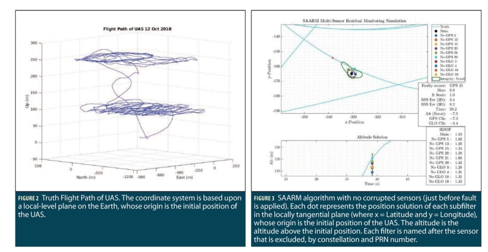
A dataset was collected during an unmanned aerial system (UAS) flight test conducted by the ANT Center at Camp Atterbury, IN. Measurement data from approximately 27 minutes of one flight scenario is used here. The aircraft flew at predominately two different altitudes: 250 and 100 meters above the local surface. The truth dataset was derived using the ANT Center’s Scorpion framework to process measurements from several sensors, including inertial measurements, to arrive at a standard EKF solution at a given timestamp. This solution was used as the truth trajectory. The timestamp was pulled from the UNIX system time on the computer running the Scorpion software. The plot in Figure 2 depicts the flight trajectory of the truth dataset. The origin of the coordinate system was set to the initial position of the UAS at the beginning of the data collection.
GNSS range data was collected from a GNSS receiver every 0.2 seconds in GPS time (dt = 0.2). To synchronize the truth data with the range data that was collected, the truth position data was converted to the Cartesian (Earth-Centered Earth-Fixed, ECEF) coordinate system and linearly interpolated in each dimension to match the times at which the GNSS measurements were received. To account for leap seconds, 18 seconds were added to the UNIX time to match up with the time of reception of the pseudorange measurements, which were reported in GPS time. To take advantage of a GNSS sensor’s ability to make ionosphere range corrections, the ionosphere bias was removed from the measurement prior to being processed by the SAARM subfilters. The bias was removed via the L1 Klobuchar parameters broadcast with the GPS ephemeris message. These parameters were applied to the GLONASS pseudoranges as well.
Parameters and Initializations
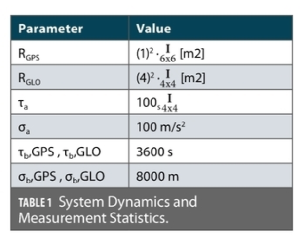
Table 1 defines the parameters for the system dynamics and measurement covariance. These values were replicated in every subfilter as they were initialized. Every subfilter was initialized with the same initial prediction error covariance (Po) data.
The initial state estimation was set to zero, where the origin of the position coordinate system is the initial truth position, although unknown to the filter. The filter processed pseudorange measurements with the ionosphere removed, and with the satellite positions precalculated and converted to the local-level frame. The ARMAS integrity filter requires the selection of two key parameters by the user: the monitoring period, M in seconds; and probability of false alarm. For this dataset, was set to 30 s; the α for each individual filter was set to 6.67×10⁻⁶.

Flight Test Results
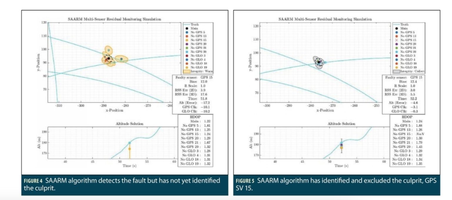
The SAARM algorithm was post-processed from data collected from a GNSS receiver’s raw pseudorange measurements during the ANT Center’s flight test. It is assumed that no previous bias, with the exception of minor multipath, was incorporated into the receiver’s measurements. A growing range bias of 1 m every second (i.e. 0.2 m every 0.2 seconds) was added to one SV’s measurement to test the SAARM algorithm to detect and exclude this measurement. The 2D and Altitude GPZ, as well as the detection and exclusion of one culprit SV measurement, are illustrated in Figures 3 through 5. The names of the subfilters are based upon the particular constellation and PRN of the excluded measurement. The values of x and y are based upon the distance from the initial truth position of the UAS, x for Latitude, y for Longitude. The horizontal dilution of precision (HDOP) values are also depicted, along with the faulty sensor, the distance of the bias added to the faulty sensor, as well as the 2D,3D, and altitude errors from the truth.
Figure 3 depicts SAARM just before the fault is applied, depicted by the small red triangle in the truth path. Figure 4 depicts the detection of a faulty sensor, but SAARM has not yet identified the culprit. Figure 5 depicts SAARM after the culprit has been identified and excluded. The observed images demonstrate that the SAARM algorithm is able to work with real-world measurements.
The faulty sensor as well as the biases that are applied, the time elapsed since the beginning of the data set, and 2D and 3D errors from the truth are depicted in the middle-right window. HDOP values for each subfilter are depicted in the lower right, providing useful data to assist with one particular phenomenon observed throughout the running of the ARMAS filter.
Analysis
HDOP data provides insight into the observability of the system, although it is not exactly observability. The correlation between geometry and observability is especially strong in this experiment, as the only measurements in the filter are GNSS measurements. When there is weak or only partial observability, the subfilter solutions can vary dramatically and can seem to “swing” wildly from one solution to another. Loss of observability also removes the power of this integrity approach to detect and remove sensor problems. An example scenario of when this might happen is when there is low availability of GNSS satellites and, due to the relative geometry, two or more satellites can appear close together, effectively reducing the number of satellites. Effects of this phenomenon can be observed when running the SAARM algorithm with only GPS satellite measurements.
To illustrate, the SAARM algorithm compares two different scenarios near the same time: one incorporating only 6 GPS SV measurements, and the other that includes 4 GLONASS SV measurements for a total of 10 SV measurements. Figure 6 shows the first scenario with bad geometry while Figure 7 shows the latter scenario with better geometry.
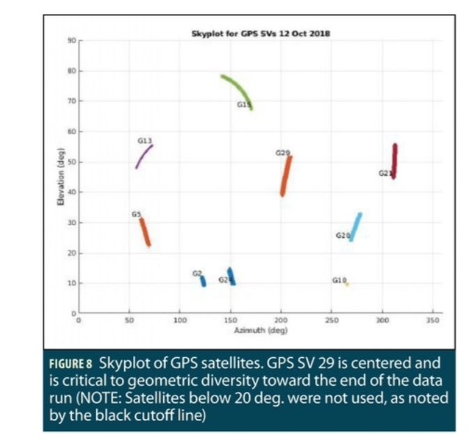
The measurements from satellites below 20 degrees elevation were not used due to greater multipath and increased measurement dropouts. The 20-degree cutoff line is indicated in Figure 6. As illustrated in Figure 6, the subfilter excluding GPS PRN 29 suffers from bad geometry, as the HDOP is greater than 10. The bad geometry causes intermittent integrity warnings due to false alarm errors, although the algorithm did not outright exclude any sensors.
Careful observation of the skyplot in Figure 8 details why this occurs: Excluding PRN 29 removes the middle satellite from the overall geometry. The remaining satellites are not well spread out from the perspective of the GNSS receiver on the UAS. Therefore, for the geometry depicted in this dataset, when only incorporating the six GPS satellites above 20 degrees elevation, SV 29 is the most critical to maintaining a good geometry. This SV’s critical importance is underscored by the low availability of GNSS-only measurements above 20 degrees elevation. The remaining subfilters that excluded other satellites did not suffer from this issue. In general, this is a violation of SAARM’s position state observability assumption for all subfilters.
Observability
The ARMAS framework with SAARM was originally conceived and simulated with basic 2D sensors and assumed fully overlapping position observability in every subfilter within the FDE subfilter layer. Pseudoranges are extracted from six SVs for processing in ARMAS as individual pseudorange sensors. During the analysis of the 27-minute flight test dataset, it is clear that the latter half of the flight test dataset contains numerous sensor dropouts. Initial analysis reveals that a sensor dropout causes spurious behavior in ARMAS. SAARM is unable to provide a subfilter consensus to identify a failed sensor when the FDE subfilter layer loses overlapping position state observability. In other words, SAARM can detect a sensor fault but cannot exclude the faulty sensor if even a single FDE layer subfilter loses position state observability due to dropout, poor geometry, etc.
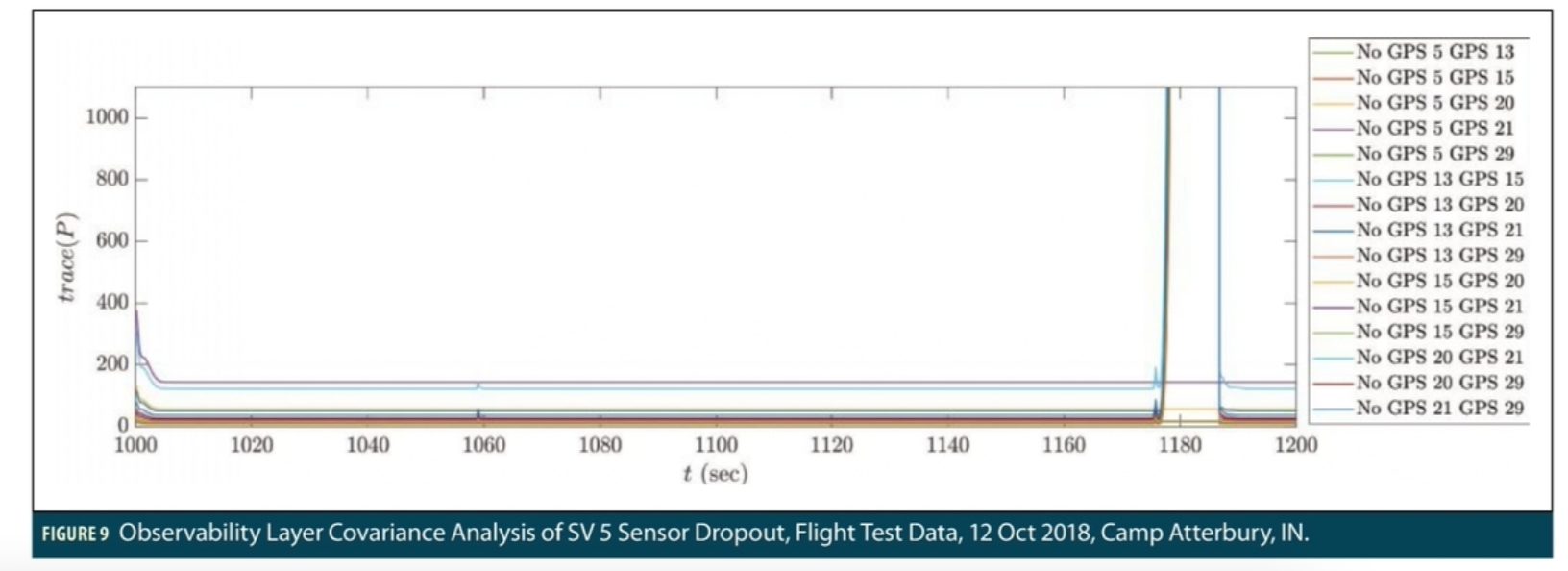
Since the initial simulation of ARMAS was performed with fully overlapping position state observability in the FDE layer, this problem was not identified in development. Figure 9 shows a local covariance analysis of the observability layer subfilters. For the observability analysis, a second integrity layer of subfilters is added, similar to a case when one would expect two faulty sensors. There are now 2 integrity layers consisting of 15 subfilters in the observability layer for 6 pseudorange sensors. Each subfilter in the observability layer is informed by 4 unique pseudorange sensors, the minimal case for a stable 3D solution.
In other words, a single pseudorange sensor dropout results in the loss of position state observability and is evidenced by an increase in the trace(Pxyz). At approximately t = 1175 sec, SV 5 experiences a transient dropout which affects all but 5 of the observability layer sub-subfilters (No GPS 5 GPS 13, No GPS 5 GPS 15, No GPS 5 GPS 20, No GPS 5 GPS 29). As a side note, these observability layer sub-subfilters would form the new FDE layer if GPS 5 were excluded from the monitoring mode. This analysis forms the genesis of local observability research at the subfilter level to preserve the consistency of the FDE layer and the integrity functions of ARMAS in the event of a single simultaneous sensor failure.
Conclusions and Future Work
Processing data from a flight test, the SAARM algorithm processed pseudorange measurements with one measurement corrupted with a growing range bias of 1 meter per second. The algorithm successfully detected and excluded this corrupted satellite measurement with no false exclusions before or after this time. Observing the geometry of certain subfilters gives further insight into the factors leading to possible false alarm errors in the event of low availability due to jamming, spoofing, or operating in urban or other obscured environments. Incorporating additional GNSS signals through adding the GLONASS constellation alleviated the issue of bad geometry. Insight into observability can be acquired through adding another integrity layer.
The ARMAS framework and SAARM algorithm can perform fault detection and exclusion with real-world data fused from multiple GNSS constellations and support further research and applications. Future work will incorporate sensors such as ranging radios, inertial measurement units, lidar and velocity sensors into ARMAS. These sensors will update at different rates and will thus test ARMAS with real-world asynchronous measurements. Research will also explore estimating the attitude and utilization of error states within SAARM. The ARMAS framework will also incorporate all five modes of operation to test the re-calibration or resilient sensor recovery of failed sensors. One such method to test ARMAS is a bias that would be present and then disappear so that the sensor would return to monitoring mode. Follow-on applications would then be to apply the ARMAS framework in real-time to detect bad measurements to improve navigation integrity. 
Acknowledgements
The authors wish to thank Lt. Col Juan Jurado of the U.S. Air Force Test Pilot School for developing the ARMAS framework and Dr. John Raquet for providing guidance and reviewing the material.
Authors

Andrew Appleget is a research engineer at the Autonomous Navigation and Technology (ANT) Center at the Air Force Institute of Technology (AFIT) at Wright-Patterson Air Force Base (WPAFB). He received his MSEE from Ohio University.

Robert C. Leishman is Director of the ANT Center at AFIT and research assistant professor in the Dept. of Electrical & Computer Engineering. His research spans autonomous vehicles, robust alternative navigation, image processing, sensor fusion,and control. He has a Ph.D. in mechanical engineering from Brigham Young University.

Maj. Jonathon Gipson is a Ph.D. candidate at the Air Force Institute of Technology and an experienced flight test engineer in the Air Force. He is a graduate of the Air Force Test Pilot School.


