We are witnessing a space renaissance. Tens of thousands of broadband low Earth orbit (LEO) satellites are expected to be launched by the end of this decade. These planned megaconstellations of LEO satellites along with existing constellations will shower the Earth with a plethora of signals of opportunity, diverse in frequency and direction. These signals could be exploited for navigation in the inevitable event that GNSS signals become unavailable (e.g., in deep urban canyons, under dense foliage, during unintentional interference, and intentional jamming) or untrustworthy (e.g., undermalicious spoofing attacks).
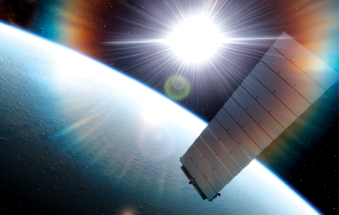
The ambitious and glorified image of an Earth connected through a web woven from low-Earth orbit (LEO) satellites is taking the world by storm, promising high-resolution images; remote sensing; and global, high-availability, high-bandwidth and low-latency Internet. Many corporations, such as Orbcomm, Globalstar, and Iridium, made haste in securing their position in space as LEO constellations were born. With the recent developments in satellite technology, reduction in launch costs and commercialization of LEO megaconstellations, LEO satellites’ popularity is soaring. Major technology giants such as SpaceX, Amazon and OneWeb rush to enter this field by launching and scheduling the launch of thousands of satellites for Internet connectivity and communication purposes.
The promise of utilizing LEO satellites for navigation has been the subject of recent studies [1]–[4].
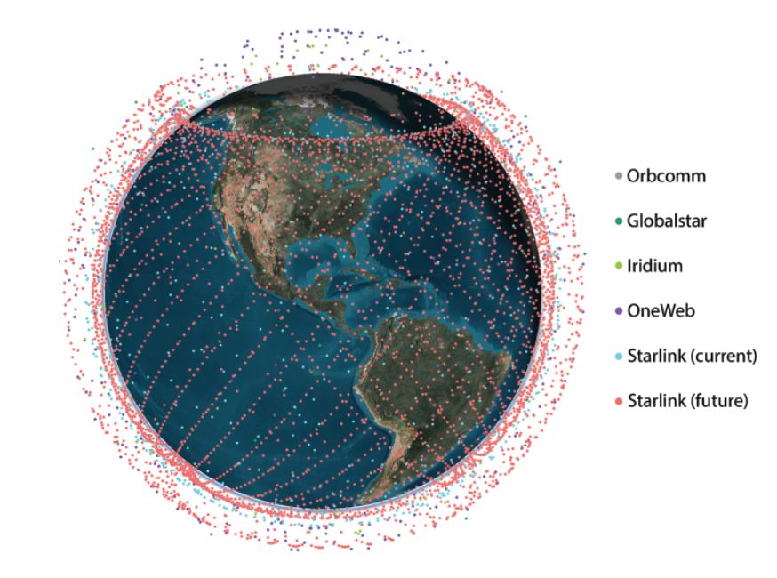
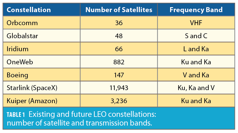
While some studies call for tailoring the transmission protocol to support navigation capabilities [5], other studies propose to exploit the transmitted signals for navigation in an opportunistic fashion [6]. The former studies allow for simpler receiver architectures and navigation algorithms. However, they require significant investment in satellite infrastructure and spectrum allocation, the cost of which private companies; such as OneWeb, SpaceX, Amazon, among others; which are planning to aggregately launch tens of thousands of satellites into LEO (see Figure 1 and Table 1) may not be willing to pay.
Moreover, if the aforementioned companies agree to that additional cost, there will be no guarantees that they would not charge for “extra navigation services.” As such, exploiting LEO satellite signals opportunistically for navigation becomes the more viable approach. This article studies opportunistic navigation with the Starlink megaconstellation of LEO satellites.
To address the limitations and vulnerabilities of GNSS, opportunistic navigation has received significant attention over the past decade or so. Opportunistic navigation is a paradigm that relies on exploiting ambient radio signal of opportunity (SOPs) for positioning and timing [7]. Besides LEO satellite signals, other SOPs include AM/FM radio, digital television, WiFi, and cellular, with the latter showing the promise of a submeter-accurate navigation on unmanned aerial vehicles (UAVs) [8] and meter-level navigation on ground vehicles [9],[10].
LEO satellites possess desirable attributes for navigation. First, LEO satellites are around twenty times closer to Earth compared to GNSS satellites that reside in medium-Earth orbit (MEO), making LEO satellites’ received signals significantly more powerful than GNSS (more than 30 dB). Second, LEO satellites orbit the Earth at much faster rates compared to GNSS satellites, making LEO satellites’ Doppler measurements attractive to exploit.
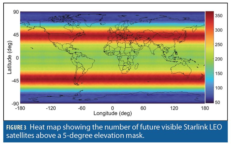
Third, LEO megaconstellations will shower Earth with signals diverse in frequency, improving robustness to interference and cyberattacks. Fourth, LEO satellites will provide virtually a blanket cover around the globe, yielding low geometric dilution of precision (GDOP), which in turn gives more precise position estimates. These are not ungrounded promises. As of mid-2021, SpaceX has launched over 1,600 Starlink satellites into LEO, with the total being projected to be up to 42,000 satellites, 12,000 of which are already approved by the Federal Communications Commission (FCC).
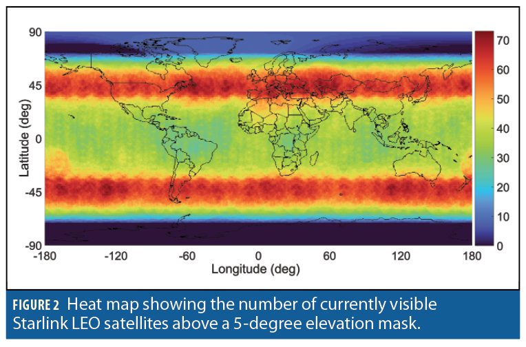
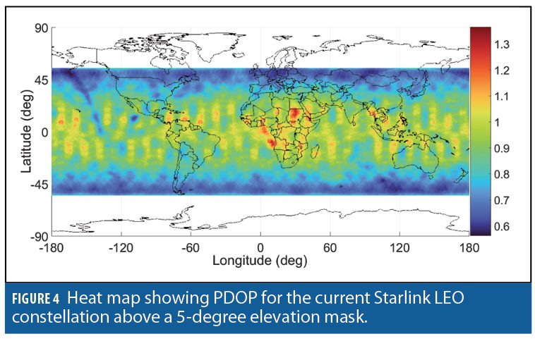
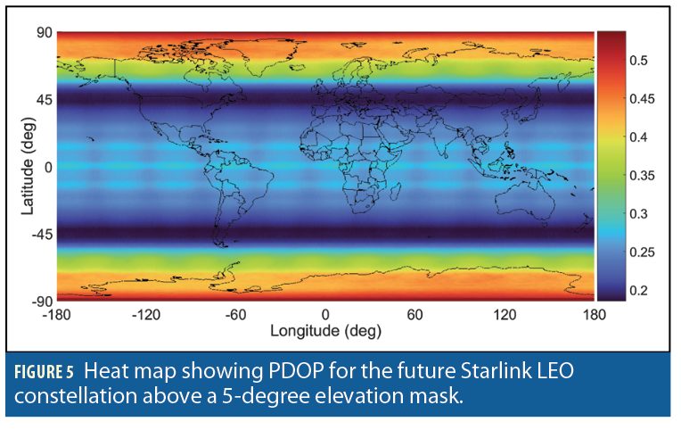
Figure 2 and Figure 3 show a heat map of the number of currently visible versus future Starlink LEO satellites, respectively, above an elevation mask of 5 degrees. Figure 4 and Figure 5 present heat maps of the position dilution of precision (PDOP) for the current versus future Starlink constellation, respectively.
However, there is no such thing as a free lunch. A multitude of challenges must be addressed to be able to exploit LEO satellite signals in an opportunistic fashion.
First, since LEO satellites are not designed for navigation purposes, they do not necessarily transmit their satellites’ ephemerides, and in occasions that they do, we might not have access to such data as non-subscribers. The position and velocity of a satellite can be parametrized by its Keplerian elements. These elements, along with some other information about a satellite’s states, can be found in two-line element (TLE) files, which are tracked and publicly published on a daily basis by the North American Aerospace Defense Command (NORAD) [11]. However, utilizing these elements in determining the satellites’ orbits introduces errors on the order of kilometers, as these elements are dynamic and deviate due to several sources of perturbing forces, which include atmospheric drag, the Earth’s oblateness causing a non-uniform gravitational field, solar radiation pressure, and other sources of gravitational forces (e.g., the Sun and the Moon) [12]. Furthermore, with Starlink satellites orbiting at very low altitudes, the effect of these forces is amplified.
Second, unlike GNSS satellites, LEO satellites are not necessarily equipped with atomic clocks, nor they are as tightly synchronized. The stability of LEO satellites’ clocks and their synchronicity are unknown. In contrast to GNSS, where the satelites’ clock errors are periodically transmitted to the receiver in the navigation message, such information is unavailable to the receiver.
Finally, LEO satellites are owned and operated by private entities, which adopt proprietary transmission protocols; making their signals “mysterious” for non-subscribers. As such, to exploit these signals, we need to build specialized receivers that are capable of extracting navigation observables.
Navigation with Starlink Satellites
Here, we present two approaches to exploit unknown Starlink signals for navigation. The first approach relies on the single or multiple carrier signals transmitted by Starlink satellites. An adaptive Kalman filter (KF)-based phase-locked loop (PLL) algorithm is used in the first approach to extract carrier phase observables from received satellite signals. In the second approach, Starlink signals are acquired and tracked without assuming any prior knowledge on the signal. This approach considers a more generic model for the transmitted synchronization signals to provide Dopplernavigation observables.
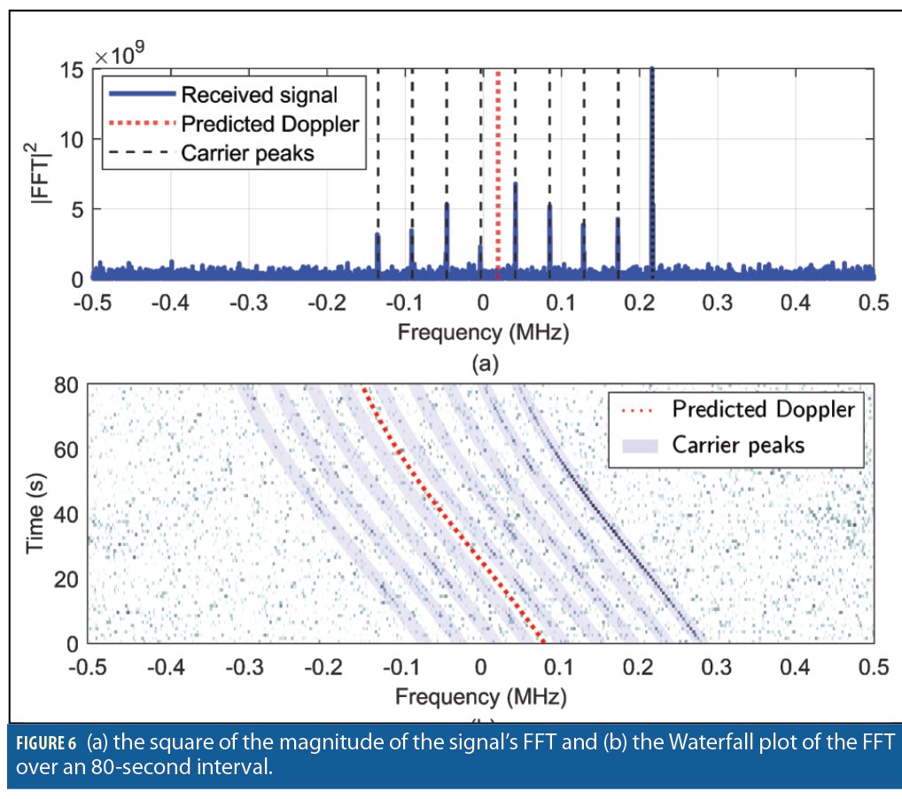
Extracting Carrier-Phase Observables. (Approach 1) A look at the magnitude of the fast Fourier transform (FFT) of the Starlink downlink signal at 11.325 GHz carrier frequency and sampling rate of 2.5 MHz shows nine peaks (Figure 6a). Figure 6b demonstrates the Waterfall plot of the FFT over an 80-second interval.
The peaks are uniformly separated by approximately 44 kHz and vary in amplitude over time. One approach to extract navigation observables from Starlink signals is to consider the peaks as carriers and develop a softwaredefined radio (SDR) to acquire and track them to generate beat carrier phase measurements. Since the receiver does not know the position of the tracked peak relative to the center frequency of the signal, a Doppler ambiguity is present, and it is accounted for in the navigation filter used to generate the position solution. The continuous-time model of the beat carrier phase is a function of
• the true range between the LEO satellite and the receiver,
• the time-varying difference between the receiver’s and LEO satellite’s clock bias, and
• the beat carrier frequency.
The clock bias is assumed to have an initial value and a constant drift. An adaptive KF-based algorithm tracks the beat carrier phase. The KF-based tracking operates similarly to Costas loops, except that the loop filter is replaced with a KF, where the measurement noise variance is varied adaptively. More details are discussed in [13].
Estimating the Synchronization Signal. (Approach 2) In most communication systems, a periodic signal is transmitted for synchronization purposes, e.g., spreading codes in 3G code division multiple access (CDMA) and primary synchronization signal (PSS) in 4G LTE and 5G. Unlike data, the synchronization signals are periodic. One can model the Starlink downlink signal as an unknown periodic signal. The detection of unknown periodic signals in the presence of noise and interference falls into the paradigm of matched subspace detectors, which has been studied in the detection literature.
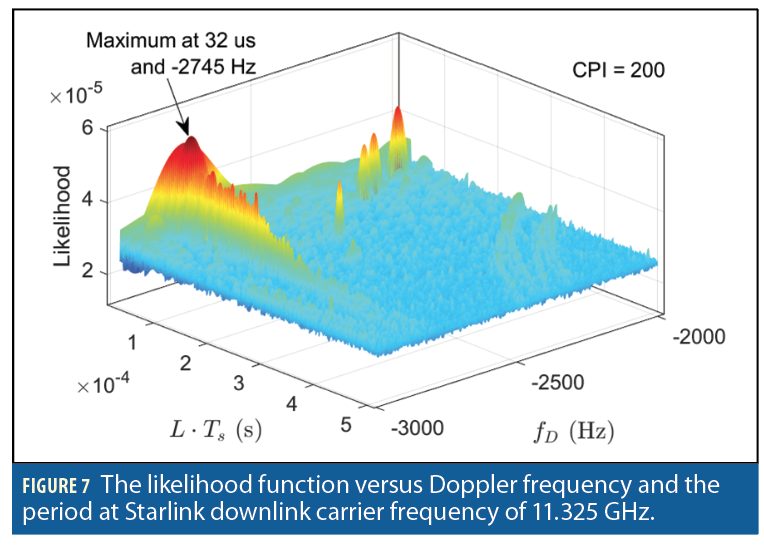
The second approach consists of two main stages: acquisition and tracking. In the acquisition stage, an estimate of the parameters of the synchronization signal and its period, denoted by L, along with an initial estimate of the Doppler frequency fD is produced. The acquisition stage is modeled as a binary hypothesis testing problem as:
Solving the detection problem produces a likelihood function which involves a two-dimensional search over the Doppler frequency and period. Figure 7 demonstrates the likelihood in terms of Doppler frequency and the period for Starlink downlink signals in the acquisition stage.
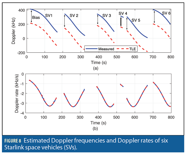
After producing these initial estimates in the acquisition stage, the estimated Doppler frequency is tracked using a Doppler tracking algorithm. To capture the high dynamics of Starlink LEO satellites, a linear chirp model is considered. More precisely, it is assumed that during the coherent processing interval (CPI), the Doppler is a linear function of time. An FFT-based chirp parameter tracking is used to track the chirp parameters which are the Doppler frequency and Doppler rate. Figure 8 demonstrates the tracked Doppler frequencies and Doppler rates of six Starlink satellites transmitting at 11.325 GHz versus those predicted from TLE files. The estimated Doppler frequencies have a constant bias compared to those predicted from TLE. This bias is present because the exact carrier frequency of the transmitted signals is unknown. This constant bias is estimated in the navigation filter. More details are discussed in [14].
Starlink LEO Ephemerides Error
One source of error to consider when navigating with LEO satellite signals arises from imperfect knowledge of the LEO satellites’ ephemerides. This is due to time-varying Keplerian elements caused by several perturbing accelerations acting on the satellite. Mean Keplerian elements and perturbing acceleration parameters are contained in publicly available TLE files. The information in these files may be used to initialize simplified general perturbations (SGP) models, which propagate LEO satellite’s orbit. SGP propagators (e.g., SGP4 [15]) are optimized for speed by replacing complicated perturbing acceleration models that require numerical integrations with analytical expressions to propagate a satellite posi-tion from an epoch time to a specified future time.
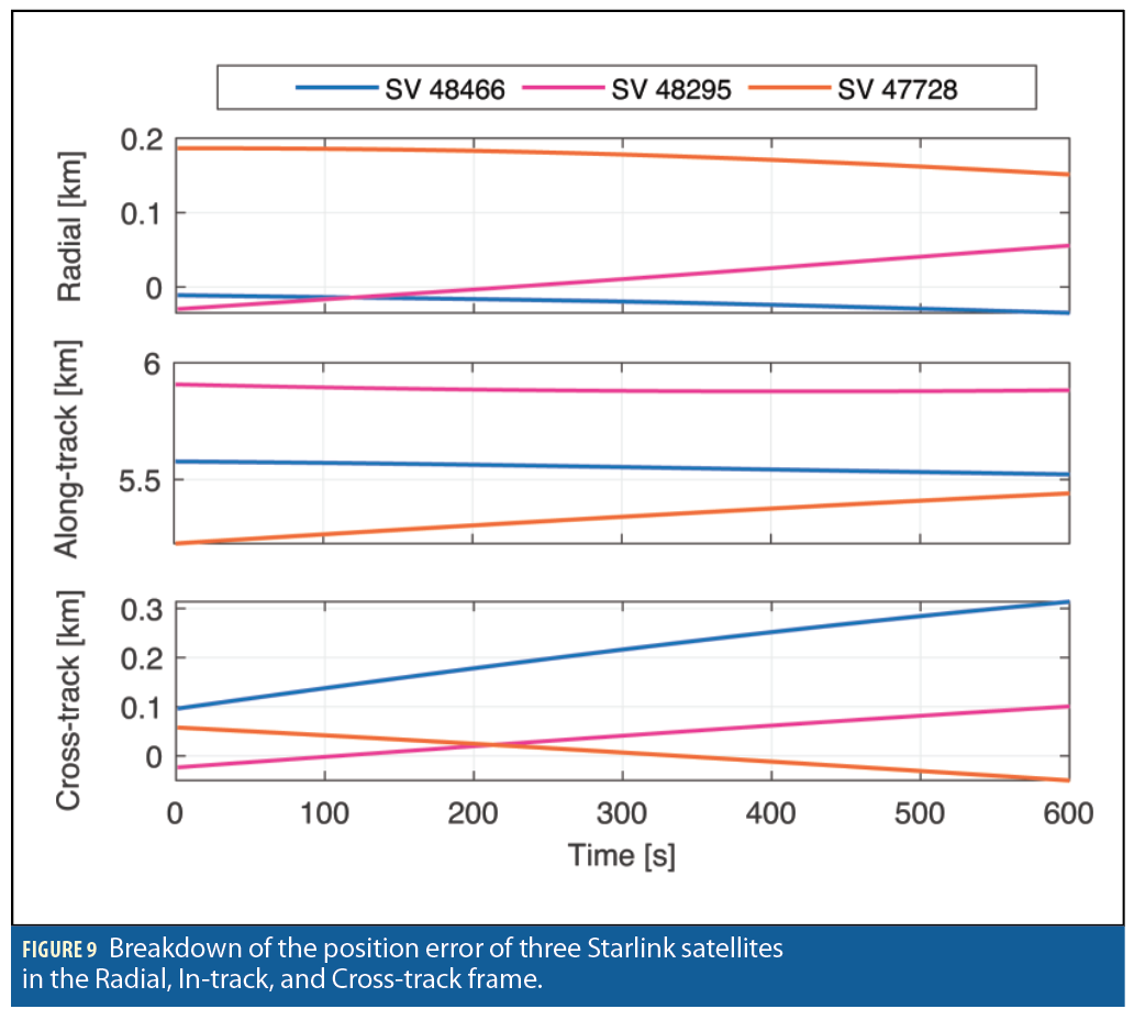
The tradeoff is in satellite position accuracy: the SGP4 propagator has around 3 km in position error at epoch and the propagated orbit will continue to deviate from the true one until the TLE files are updated the following day. Figure 9 shows the breakdown of the position error of three Starlink satellites in the radial, along-track and cross-track frame. The errors are generated by propagating Starlink satellites using SGP4 and comparing to a “ground truth,” generated by the High Precision Orbit Propagator (HPOP), which was initialized using the state vector published by Starlink. Figure 9 shows that most of the error reside along the track. More details are discussed in [16],[17].
Positioning with Starlink Carrier Phase and Doppler Measurements
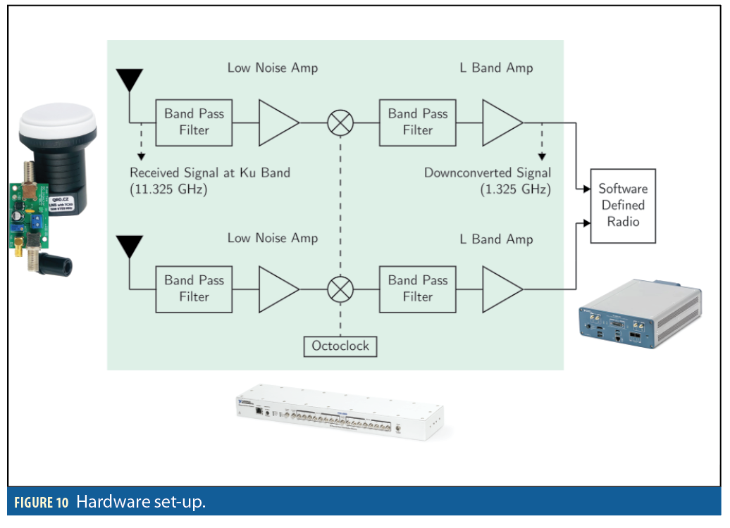
This section presents the first stationary positioning results with Starlink signals. A National Instruments (NI) universal software radio peripheral (USRP) 2945R was equipped with two consumer-grade antennas and low-noise block (LNB) downconverters to receive Starlink signals in the Ku-band from two different angles. An octo-clock was used to synchronize the USRP clocks and the downconverters. The sampling rate was set to 2.5 MHz and the carrier frequency was set to 11.325 GHz, which is one of the Starlink downlink frequencies. Figure 10 shows the hardware setup.
A weighted nonlinear least-squares (WNLS) estimator was used to estimate the receiver’s position using the six detected Starlink satellites. To account for ephemeris errors, the TLE epoch time for each Starlink satellite was shifted in time to minimize the error residuals.
The receiver’s position was initialized as the centroid of all Starlink satellite positions, projected onto the surface of the Earth, yielding an initial position error of 179 km. The clock biases and drifts were initialized to zero.
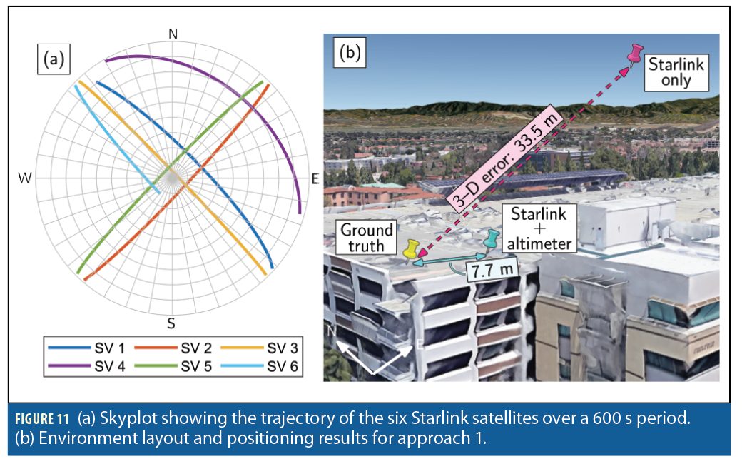
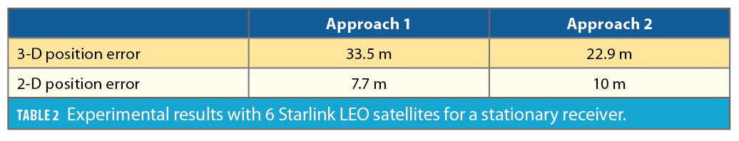
The environment layout and the positioning results are shown in Figure 11 and Table 2, respectively. The 3–D position error was found to be 33.5 m and 22.9 m for Approach 1 and 2, respectively. Upon equipping the receiver with an altimeter (to know its attitude) the 2–D position error was reduced to 7.7 m and 10 m for Approach 1 and Approach 2, respectively. More details are discussed in [13],[14].
Differential Doppler Positioning
A common approach to compensate for ephemeris errors, ionospheric and troposheric delays, clock errors, and other common model errors is to employ a differential framework, composed of a base and a rover. In differential Doppler positioning, the rover estimates its states by subtracting its Doppler measurements to Starlink satellites from Doppler measurements to the same satellites made by a base receiver with known position. This leads to fewer unknown terms that need to be estimated and to reducing the effect of common mode errors. More details are discussed in [18].
Experimental Results with Starlink Differential Doppler Measurements
This section presents experimental results of positioning with differential Doppler measurements from Starlink LEO satellites.
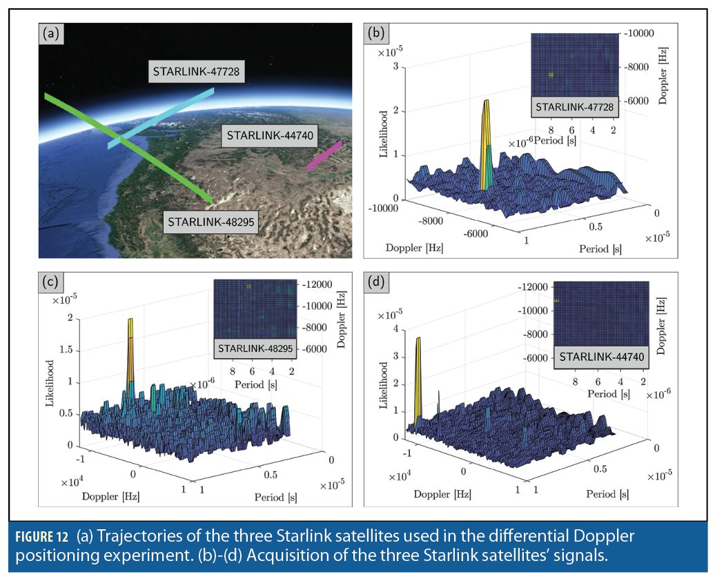
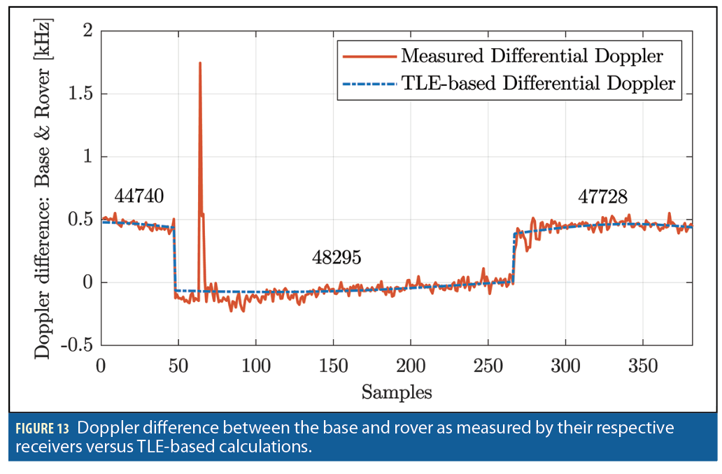
A stationary scenario is considered in which the base was equipped with an Ettus E312 USRP with a consumer-grade antenna and LNB downconverter to receive Starlink signals in the Ku- band, and the rover was equipped with USRP 2974 with the same downconverter. The Octoclocks were used to synchronize between the USRPs’ clocks and the downconverters at the base and at the rover. The sampling rate was set to 2.5 MHz, and the carrier frequency was set to 11.325 GHz. Over the course of the experiment, the receivers on-board the base and the rover were listening to 3 Starlink satellites: Starlink 44740, 48295, and 47728. The satellites were visible for 320 seconds. Figure 12shows the likelihood as a function of the Doppler frequency and period of Starlink downlink signals. The CPI was set to be 200 times the period. It can be seen that three Starlink LEO satellites were detected in the acquisition stage. Figure 13 shows the measured differential Doppler for the three satellites. The spike in the estimated differential Doppler is due to channel outage and burst error, which is common in satellite communications.
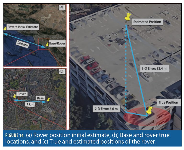
The distance between the base and the rover was 1.004 km. The rover’s initial estimate was approximately 200 km away from its true position. Upon employing the differential Doppler positioning framework, the 3–D position error was found to be 33.4 m, while the 2–D position error was 5.6 m. Figure 14 shows the positions of the base and the rover as well as the rover’s initial estimate and its final 3–D and 2–D estimates.
Simultaneous LEO Satellite Tracking and Ground Vehicle Navigation
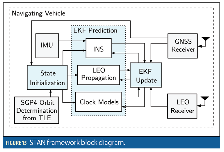
Whether navigating on water, over land or in air, most vehicles traditionally rely on a GNSS-aided inertial navigation system (INS). This GNSS/INS integration—which can be loose, tight, or deep—provides a navigation solution that benefits from both the short-term accuracy of the INS and the long-term stability of GNSS [19]. LEO satellites’ signals could be opportunistically exploited as an INS aiding source, thus serving as a complement or even an alternative to GNSS signals. GNSS satellites are equipped with highly stable atomic clocks, are synchronized across the network, and they transmit their ephemeris data and clock errors to the user in their navigation message. In contrast, LEO satellites are not designed for navigation purposes. As such, their on-board clocks are not necessarily of atomic standards nor as tightly synchronized. Moreover, LEO satellites typically do not openly transmit their ephemeris and clock error data in their proprietary signals. To remedy these challenges, the simultaneous tracking and navigation (STAN) framework was proposed, in which the navigating vehicle’s states are simultaneously estimated with the states of the LEO satellites [2],[20]. STAN employs an extended Kalman filter (EKF) to aid the vehicle’s INS with navigation observables (e.g., carrier phase and Doppler), extracted from LEO satellites’ signals in a tightly coupled fashion.
Figure 15 shows a block diagram of the STAN framework. The navigating vehicle’s statevector xv estimated in the STAN framework are the vehicle’s body frame orientation with respect to the Earth-centered Earth-fixed (ECEF) reference frame, the vehicle’s 3-D position and velocity in the ECEF frame, and the gyroscope and accelerometer biases, namely:
The mth LEO satellite’s state vector xLEOm consists of its 3-D position and velocity expressed in the Earth-centered inertial (ECI) reference frame as well as the relative clock bias and clock drift between the receiver and the mth LEO satellite, i.e.,
The state vector estimated in the STAN EKF is formed by augmenting the vehicles’ states with each LEO satellite’s states to get
Experimental Results: Ground Vehicle Navigation with Starlink and Orbcomm LEO Satellites
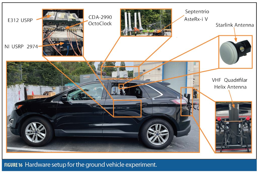
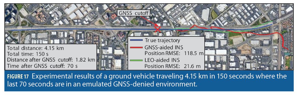
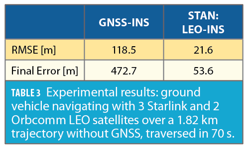
This section presents experimental results demonstrating the performance of ground vehicle navigation with 3 Starlink and 2 Orbcomm LEO satellites via the STAN framework. The vehicle was driven along the CA-55 freeway in California, USA, for 4.15 km in 150 seconds. The vehicle was equipped with a Septentrio AsteRx-I V integrated GNSS-INS system, a VectorNav VN-100 microelectro-mechanical systems (MEMS) tactical-grade inertial measurement unit (IMU), two LNBs connected to a USRP-2794 to sample Starlink satellites signals at 11.325 GHz, and a VHF antenna connected to an Ettus E312 USRP to sample Orbcomm signals at 137-138 MHz as shown in Figure 16.
During the first 80 seconds, GNSS signals were available but were fictitiously cut off for the last 70 seconds of the experiment, during which the vehicle traveled for 1.82 km. The GNSS-INS navigation solution drifted to a 3-D position root mean squared error (RMSE) of 118.5 m from the actual trajectory while the STAN LEO-aided INS yielded a 3-D position RMSE of 21.6 m. Figure 17 illustrates the true and estimated trajectories and Table 3 summarizes the navigation results.

Simulation Results: A Glimpse to the Future
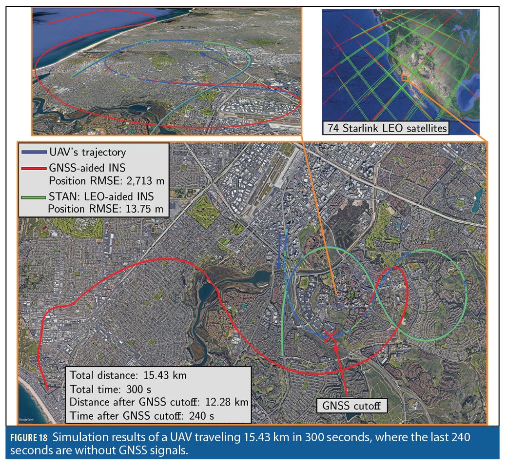
This section presents simulation results demonstrating the achievable opportunistic navigation performance with the future Starlink megasconstellation upon launching its 12,000 LEO satellites that are approved by the FCC. A fixed-wing UAV was equipped with a tactical-grade IMU, an oven-controlled crystal oscillator (OCXO), and GNSS and Starlink LEO receivers. The Starlink receiver produced Doppler measurements to visible Starlink satellites. The Starlink satellites were equipped with chip-scale atomic clocks (CSACs). The Doppler measurement noise variances ranged between 500–1,500 Hz2 , which were varied based on the predicted carrier-to-noise ratio, as calculated based on the satellites’ elevation angle. The simulated UAV compares in performance to a small private plane with a cruise speed of roughly 50 m/s. The UAV flew over Irvine, California, USA for a 300-second trajectory covering 15.43 km. The trajectory consisted of a straight climbing segment, followed by a figure-eight pattern, and then a final descent into a straight segment. The UAV, initially at 1 km altitude, climbed to an altitude of 1.5 km, where it began executing rolling and yawing maneuvers before descending back down to 1 km in the straight segment. The Starlink satellite states were initialized using TLE files and the trajectories of the 74 Starlink LEO satellites used to navigate the UAV are shown in Figure 18 (the trajectories are colored in red when the satellites are outside the 20° elevation mask and in green when they are visible to the UAV). GNSS was available for the first 60 s of the flight and STAN with Starlink satellites was performed without GNSS for the last 240 s of the trajectory. Figure 18 illustrates the simulation results and Table 4 summarizes the navigation results.
Acknowledgment
This work was supported in part by the Office of Naval Research (ONR) under Grant N00014-16-1-2305, in part by the National Science Foundation (NSF) under Grant 1929965, in part by U.S. Department of Transportation (USDOT) under Grant 69A3552047138 for the CARMEN University Transportation Center (UTC), and in part by the Air Force Office of Scientific Research (AFOSR) under the Young Investigator Program (YIP) Grant.
Authors
Zaher (Zak) M. Kassas is an associate professor at the University of California, Irvine (UCI) and The Ohio State University. He is director of the ASPIN Lab and also director of the U.S. Department of Transportation Center for Automated Vehicle Research with Multimodal AssurEd Navigation (CARMEN). His research interests include cyber-physical systems, navigation systems, and intelligent transportation systems.
Mohammad Neinavaie is a Ph.D. student at UCI and a member of the ASPIN Lab. His research interests include cognitive radio.
Joe Khalife is postdoctoral scholar at the ASPIN Lab. His research interests include modeling and analysis of signals of opportunity.
Nadim Khairallah is a Ph.D. student at UCI and a member of the ASPIN Lab. His research interests include opportunistic navigation.
Sharbel Kozhaya is a Ph.D. student at UCI and a member of the ASPIN Lab. His research interests include cognitive software defined radio.
Jamil Haidar Ahmad is a Ph.D. student at UCI and a member of the ASPIN Lab. His research interests include satellite-based navigation
Zeinan Shadram is a postdoctoral scholar at the ASPIN Lab. Her research interests include modeling and analysis of signals of opportunity.


