
Novel protection level formulas, combining RAIM with solution separation and Precise Point Positioning, are applied to static, automotive, and flight scenarios. The authors of this article demonstrate that protection levels below 2 meters are achieved with reduced computational loads.
Precise Point Positioning (PPP) techniques (see J. Kouba and P. Heroux in Additional Resources) can provide centimeter accuracy without local reference stations in kinematic applications. These techniques have so far mostly been used to provide high accuracy, and it is only recently that they have been proposed to provide integrity, that is, position error bounds with a very low probability of exceeding them. There has been preliminary work on the application of integrity to PPP (P. F. Madrid et alia), but it remains a challenge to translate the benefits of PPP to accuracy while maintaining high integrity. Most of the integrity work in PPP and RTK has dealt with the ambiguity resolution process under nominal error conditions (G. Seepersad et alia; P. F. de Bakker et alia) and less on the integrity of the position solution under fault conditions. This article integrates solution separation techniques developed for Advanced RAIM (ARAIM) with PPP to produce meter-level protection levels for static, automotive and flight scenarios.
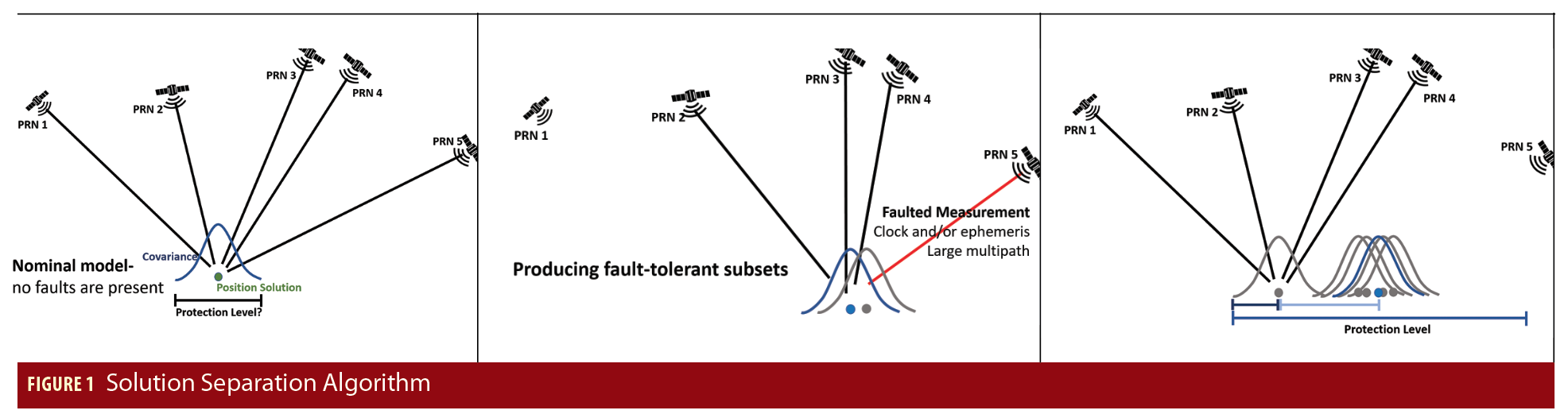
Solution separation (K. Gunning et alia) is a powerful technique for providing bounds on the error of a navigation solution. Due to its simplicity and optimality properties, it is the basis for the ARAIM user algorithm (see Additional Resources), and has been adapted for use with PPP in this work. Figure 1 shows a simple depiction of the solution separation algorithm. On the left of the figure is a navigation solution produced using five un-faulted measurements. The estimator outputs a position solution and a covariance, or predicted level of uncertainty based on the measurement models and geometry of the satellites. If one would like to produce a protection level, or a bound on the position error, one might think to simply inflate the covariance by the appropriate amount for the desired level of integrity. However, this assumes that all of the measurements are behaving according to their nominal models. This is not always the case, as faults may be present. A fault is defined as an excessively large error that could be caused by large errors in the orbit and clock estimates used, multipath, etc. In the middle of Figure 1, the measurements coming from PRN 5 are now faulted, leading to an error in the all-in-view position estimate (blue dot). The all-in-view estimate uses all measurements available. Solution separation produces solutions using fault-tolerant subsets of the measurements available. In the middle of Figure 1, the gray dot and curve represent a solution that excludes PRN 1. In other words, if there were a fault on PRN 1, then this solution would not be affected by it. This solution computation process with subsets can be repeated for all available subsets, which is shown on the right. When the faulted PRN is excluded, the computed solution is very close to the true position. The protection level can then be computed by taking the distance between our all-in-view solution and inflating it using the nominal covariance of the subset solutions. This is a very simplified description of solution separation, but it captures the essence of the process
Precise Point Positioning
PPP uses externally-provided precise orbit and clock correction inputs, along with GNSS code and carrier measurements, passed to a sequential estimator such as a Kalman filter to produce high accuracy position solutions. Typically, a PPP Kalman filter might estimate, in addition to the receiver position and clock bias, float carrier phase ambiguities and a tropospheric delay parameter. Non-integer float carrier phases are estimated rather than using resolved integer ambiguities. Performance can reach sub-decimeter level for kinematic applications, but this only occurs after convergence. Long convergence times are often cited as a negative aspect of PPP, as single-constellation PPP can require upwards of 30 minutes before high accuracy estimates are available. However, as opposed to an approach that requires local corrections such as RTK, given orbit and clock corrections, PPP is globally available, making it a very attractive high accuracy technique.
Time Savings
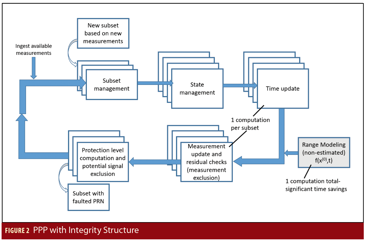
Relative to more simple navigation solution techniques like simple least-squares using carrier-smoothed code measurements, PPP is a fairly computationally demanding technique. When using solution separation in conjunction with PPP, this issue is amplified, as a separate PPP solution must be constructed for each fault-tolerant subset that is considered. Each subset solution is produced by a separate PPP Kalman filter that excludes measurements from a specific PRN or set of PRNs. Because of this, a number of steps have been taken to reduce the computational complexity of the PPP and solution separation coupling. In particular, we simplify our error models so as to reduce the number of estimated states and thereby the computational load of the Kalman filter measurement update. What this error model simplification means is that while one might have for each carrier phase measurement a state tracking the carrier phase ambiguity and another state tracking the multipath error, we simply combine those two and track a state which is the sum of the carrier phase ambiguity and the multipath error. A greater source of computational savings is that many model outputs are only computed once given the all-in-view solution as input, and the output is shared across all of the subsets. The models here are those that contribute to the predicted pseudorange and carrier phase measurements, i.e., relativity, dry troposphere, interpolated precise satellite clock and orbit, Earth solid tides, etc.
The implementation of the PPP algorithm (Figure 2) with solution separation uses an extended Kalman filter. The EKF loop starts with measurement ingestion. If any measurements are from satellites that have not been seen by the EKF before, then new subsets and states must be introduced. The new states consist of error and carrier phase ambiguity states.
The time update, wherein the state and covariance matrices are propagated from the previous time step to the current, is very straightforward. The position, velocity, and acceleration states are simply propagated forward together. All other states are assumed to be static except for the code multipath state, which is modeled as a first order Gauss-Markov process. The time update is performed individually for each subset state and covariance, but it is a relatively computationally cheap operation, as it is only matrix multiplication.
The measurement update step includes checks on the measurement residuals in order to exclude outliers. This is done by iteratively performing a measurement update and excluding measurements whose residuals exceed successively smaller thresholds until the desired small thresholds are reached. This is done because if the final thresholds are used immediately, and measurements with large error are included, those measurements can sufficiently impact the solution such that otherwise good measurements can be excluded as well. In the case of carrier phase measurements, this means reinitializing the float carrier phase ambiguity estimates unnecessarily. The exclusion of outliers here allows the fault rate at the point of the protection level computation to be kept lower than it otherwise would be, as simple things like missed cycle slips need not be included in the fault rate and are instead caught at the measurement update.
Choice of Algorithm
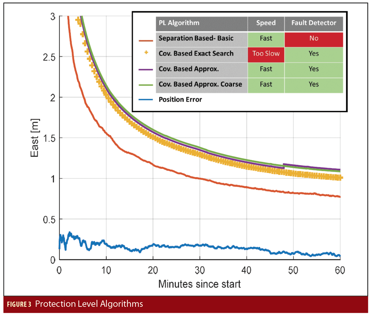
A number of different algorithms have been evaluated for their protection level performance, computational load, and fault detection abilities. Figure 3 shows the protection levels produced by four solution separation-based algorithms. Other integrity algorithms based on the sum squared of residuals have also been evaluated, and the results of this evaluation can be found in the Working Group C, Milestone 3 Report (Additional Resources). The first of the algorithms in Figure 3, called here “Separation Based- Basic,” is essentially the algorithm described earlier in this article. It is very fast and provides protection, but does not inherently detect faults, which is a feature that we desire. The next three algorithms are variations on one another, where the protection level is produced using the covariances from the subset solutions, and the position difference between the subsets is used for fault detection. The second algorithm, “cov. based exact search,” is a tight search for a protection level, but the computation time is excessive. However, the final two algorithms, which are approximations of the tight search, offer similar performance for much less computation, making them much more attractive. The algorithm chosen and used in this article is “cov. based approx.” This algorithm is based on a candidate algorithm for ARAIM solution separation. For more information on the specifics of this and the other algorithms, please again see the Milestone 3 Report in Additional Resources.
Dataset Overview
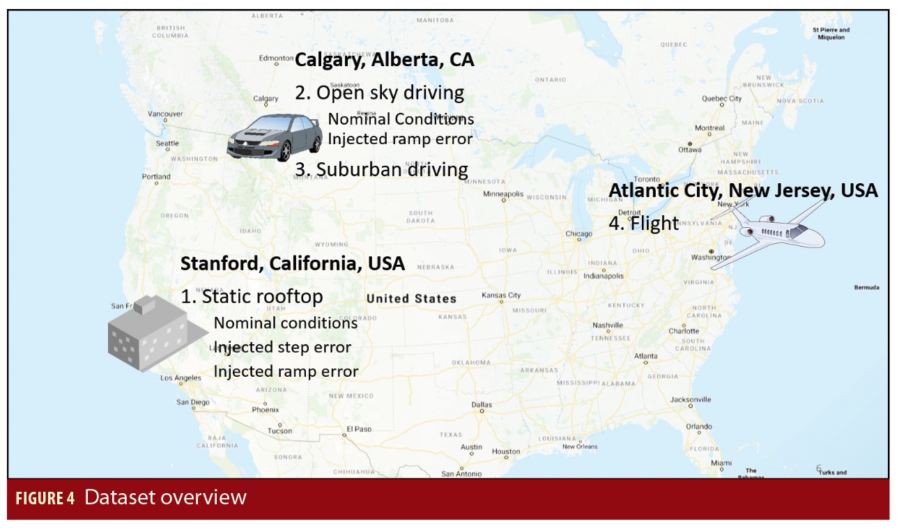
Four datasets are analyzed in the following sections: a static receiver in open sky conditions, a moving receiver in open sky road conditions, a moving receiver in suburban road conditions, and a receiver in flight conditions (Figure 4). A different receiver is used for the static, driving, and flight scenarios, but the general configurations are the same across all of them. Dual-frequency 1 Hz code and carrier phase measurements are used from GPS and GLONASS. All analyses were post-processed in MATLAB using precise clock and orbits were provided by the Center for Orbit Determination European (CODE), which is an IGS analysis center. The probability of hazardous misleading information (PHMI), which represents the probability that the error exceeds the protection level, is set to 10-7.
Static Receiver: Nominal and with Injected Faults
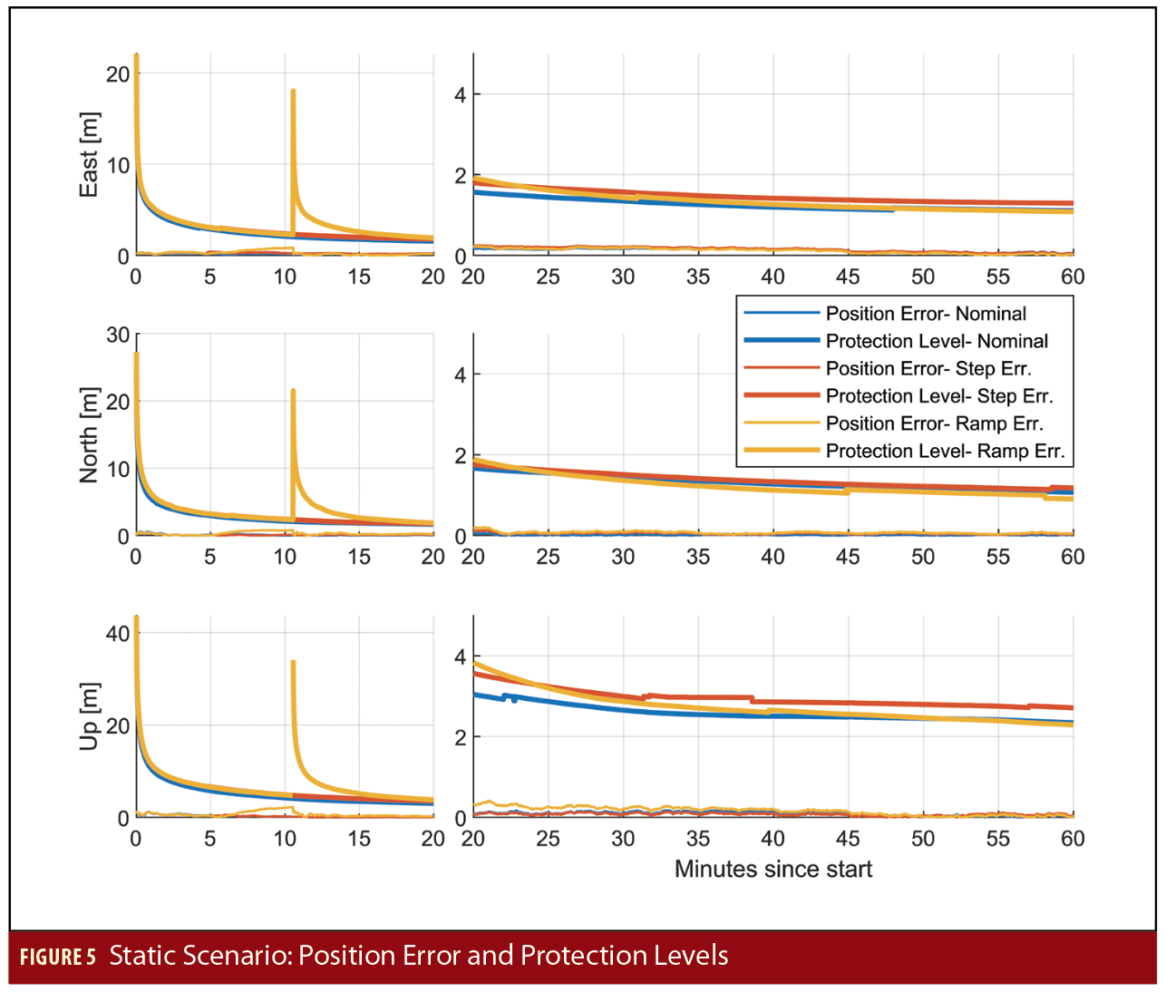
The first dataset examined is a static scenario of a receiver on top of the Aeronautics/Astronautics building at Stanford University. This survey-grade receiver is a member of the IGS network, which produces daily position solutions. The IGS daily solution serves as a static position truth for this scenario. Figure 5 shows the position errors and protection levels of the post-processed analysis of a one-hour data collection. The protection levels show the classic PPP convergence, starting out over 20 meters in each direction but converging to approximately 2 meters in the East and North directions and 4 meters in the up direction by the 20-minute mark. By the end of the run, protection levels reach 1 meter in the East and North directions and approximately 2 meters in the up direction.
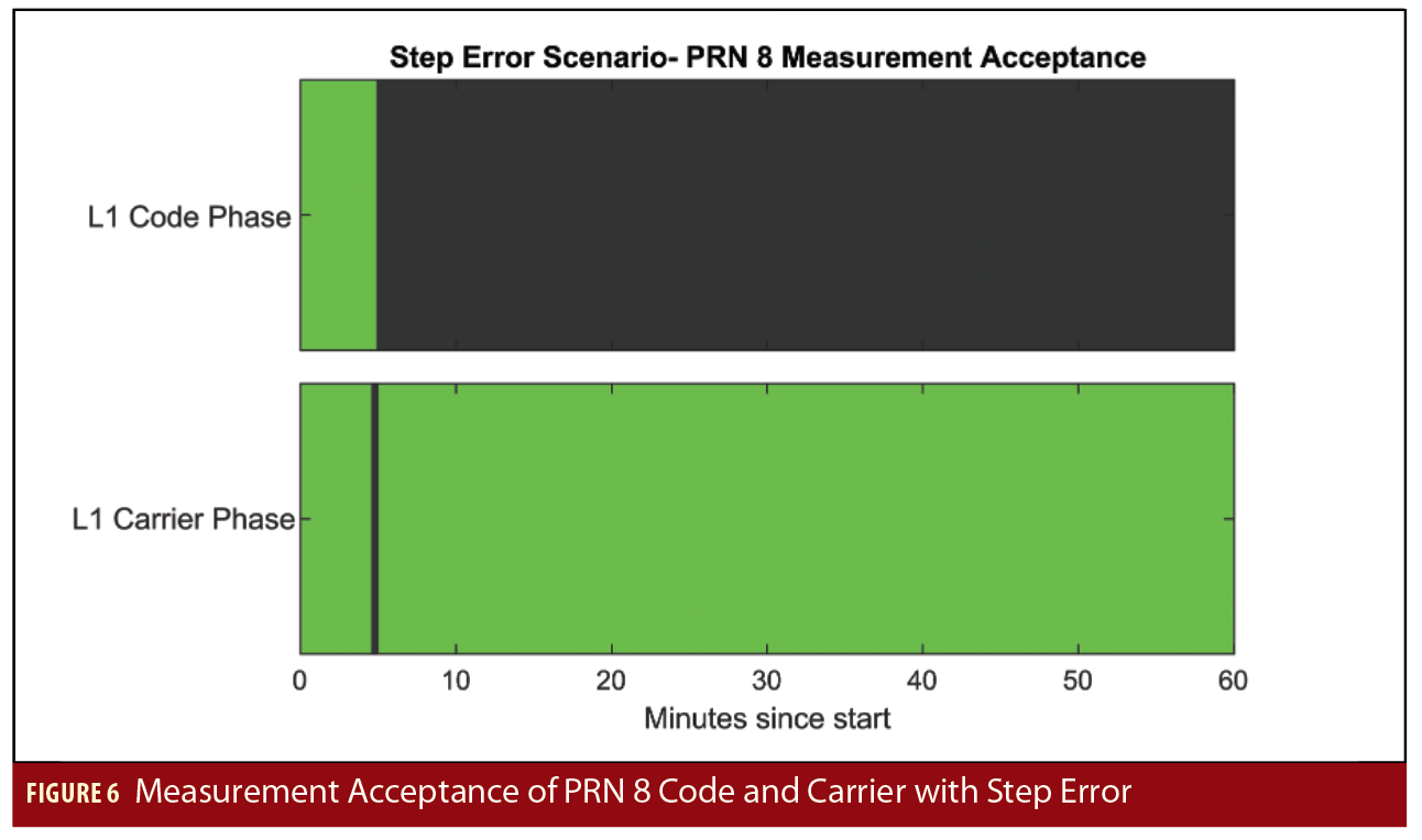
In order to examine the performance of the system under conditions where faults are present, a step and ramp fault are injected into the precise clock input for GPS PRN 8. The step fault consists of a 20-meter jump in the precise clock that begins 5 minutes into the run. The error is immediately caught at the measurement update stage, as shown in Figure 6, which plots whether or not the L1 code and carrier phase measurements are accepted (green) or rejected (black) during the measurement update. The large error in the precise clock leads to an immediate jump in the residuals of the code and carrier phase measurements. The large residuals are what lead to the measurement exclusion. In the case of the code phase, the measurements are never accepted again. However, the carrier phase measurements are accepted again after a period; in the second acceptance period, the carrier phase ambiguity estimate is offset by the 20-meter error. The position error and protection levels for this scenario are shown in Figure 5. They are largely the same as they were under nominal conditions except with a slight degradation in performance due to the weakened geometry.
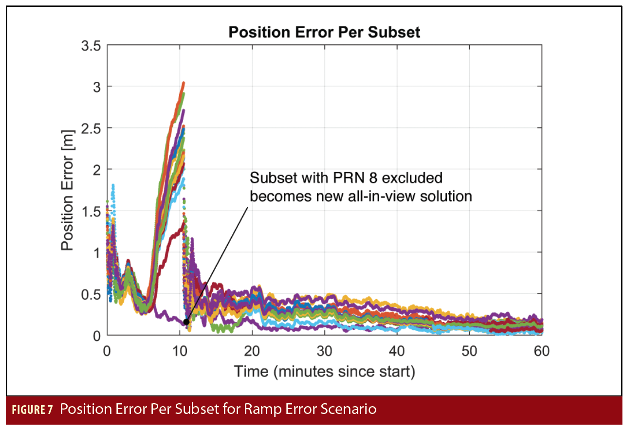
The system behaves differently under the influence of a ramp fault. The second injected fault scenario involves a ramp error of 9 meters per hour on, again, the PRN 8 precise clock. The error develops slowly enough that it is not caught by the residual checks at the measurement update step. Rather, the error is pulled into the error state estimates, and the position error of most subsets, shown in Figure 3, grows quickly. Approximately 11 minutes into the run, the fault threshold is tripped in the protection level computation. At this point, the subset with PRN 8 excluded is determined to be the fault-free subset, and the solution of that subset becomes the new all-in-view solution. The covariance and the protection levels are reinitialized, as seen in the large jumps in the protection level in Figure 7. The solution separation algorithm successfully handled both the injected step and ramp faults.
Open Sky Driving
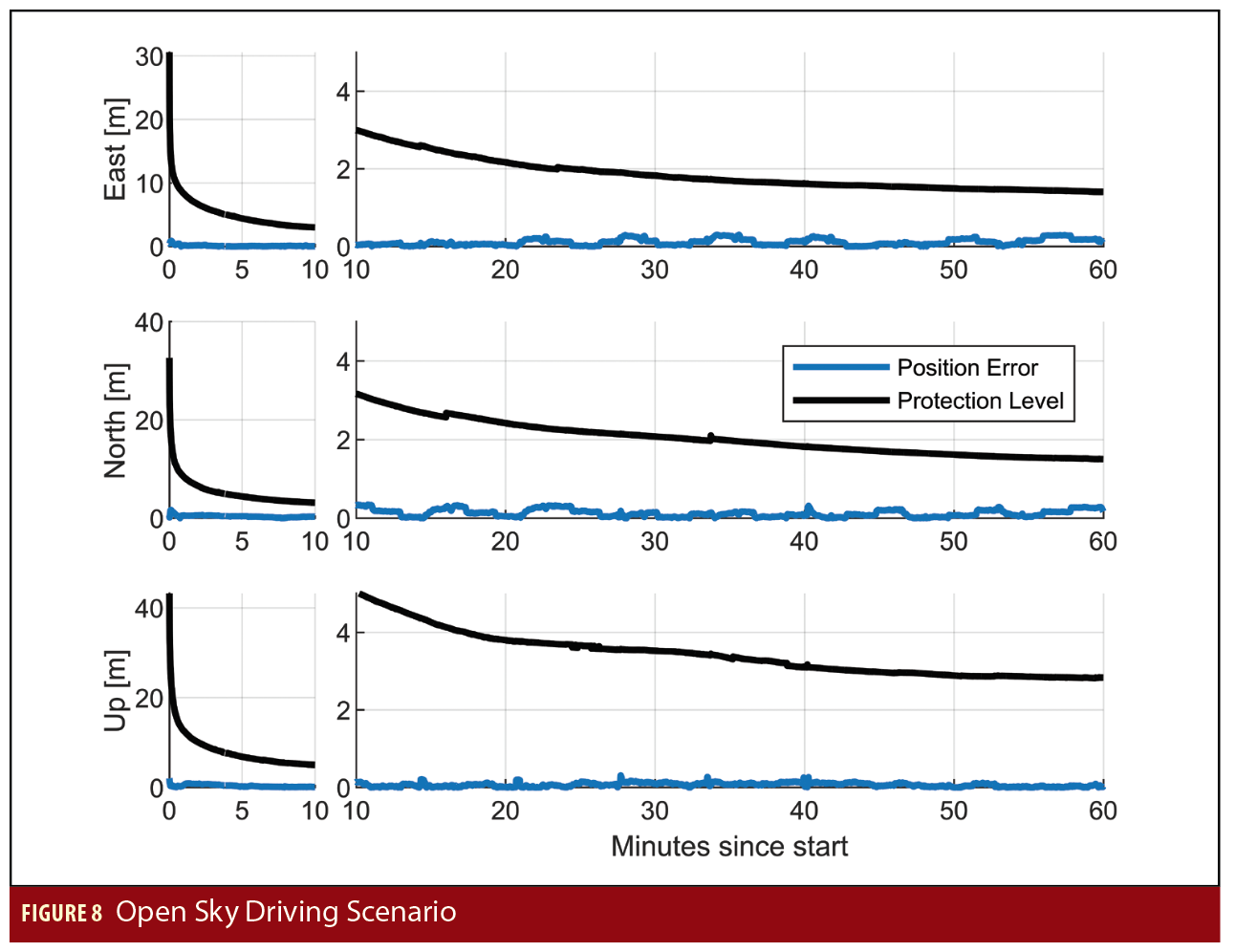
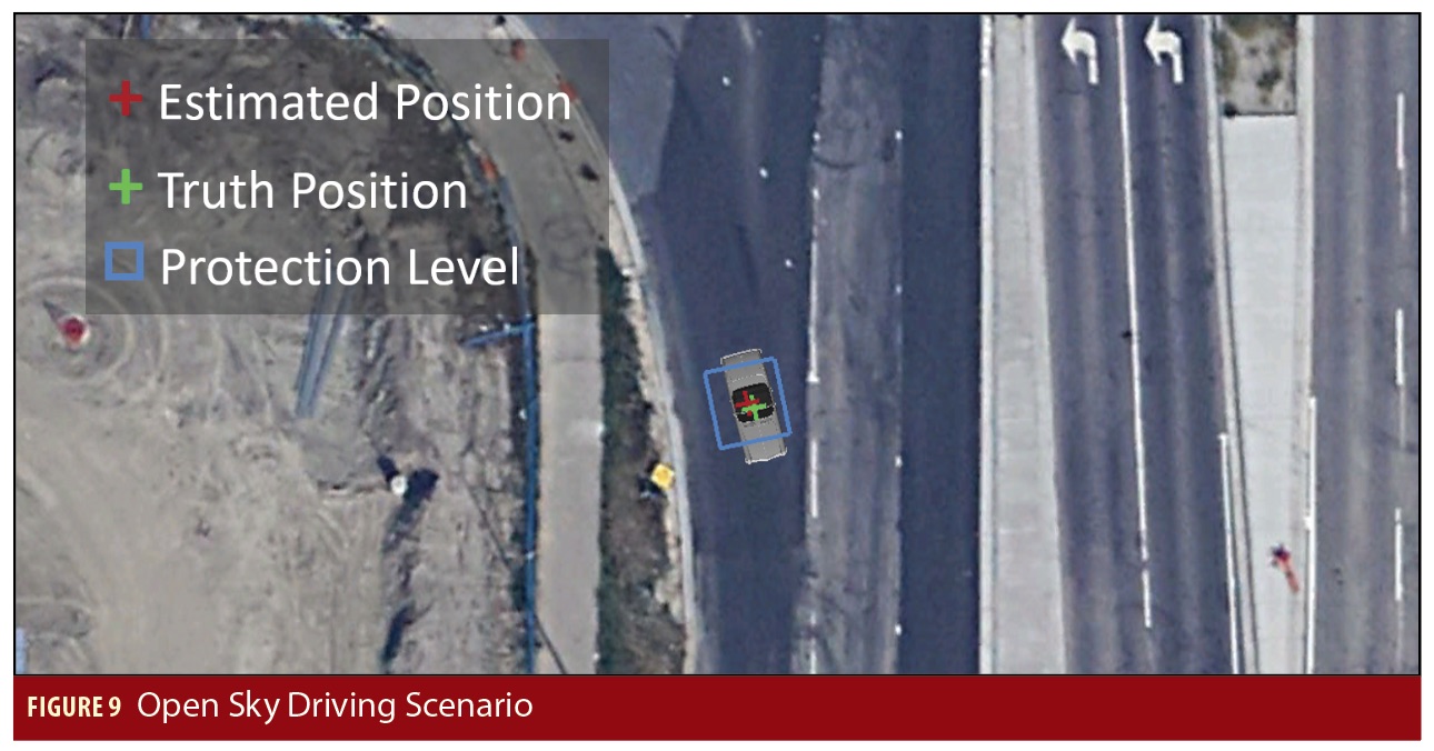
The next scenario consists of an hour-long drive under open sky conditions. The data is from an OEM just outside Calgary International Airport. The truth positions are generated from a different OEM from the same manufacturer forwards and backwards processed in conjunction with a tactical grade IMU. The measurement conditions in this scenario are generally benign, with the worst effects being from driving under large highway signs, leading to loss of lock on L2. Figure 8 shows the position error and protection levels from the PPP and solution separation system. Again, once the solution has converged, protection levels of approximately 1.5 meters are available in each of the horizontal directions, and a vertical protection level of approximately 3 meters is provided. Figure 9 shows the estimated and truth positions as well as the protection levels at the 55-minute mark of the run. Note that the protection levels offered with these techniques approach those needed for lane-level navigation.
Driving: Open Sky, Suburban
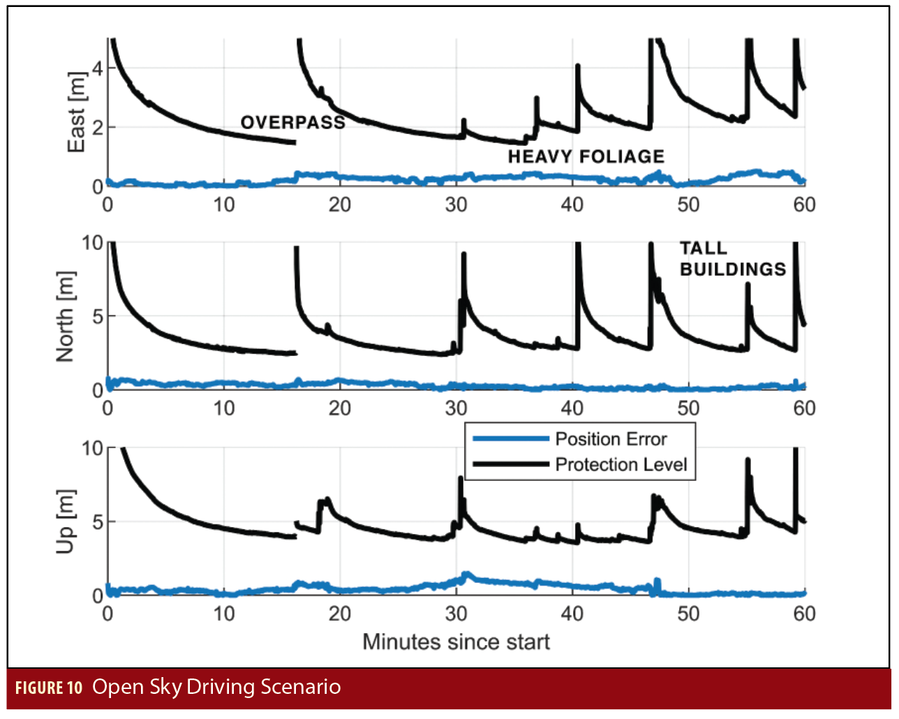
A suburban driving scenario was also analyzed. This time, the conditions are far less favorable, with various overpasses, trees, and buildings blocking most or all measurements at various points during the drive. For a PPP-based system, this means that the covariance is regularly partially or fully reinitialized as loss of lock occurs on the carrier phase measurements. This can be seen in Figure 10 in the jumps in the protection levels. Despite this, the protection levels in the horizontal directions are typically under 5 meters.
PPP vs standalone ARAIM
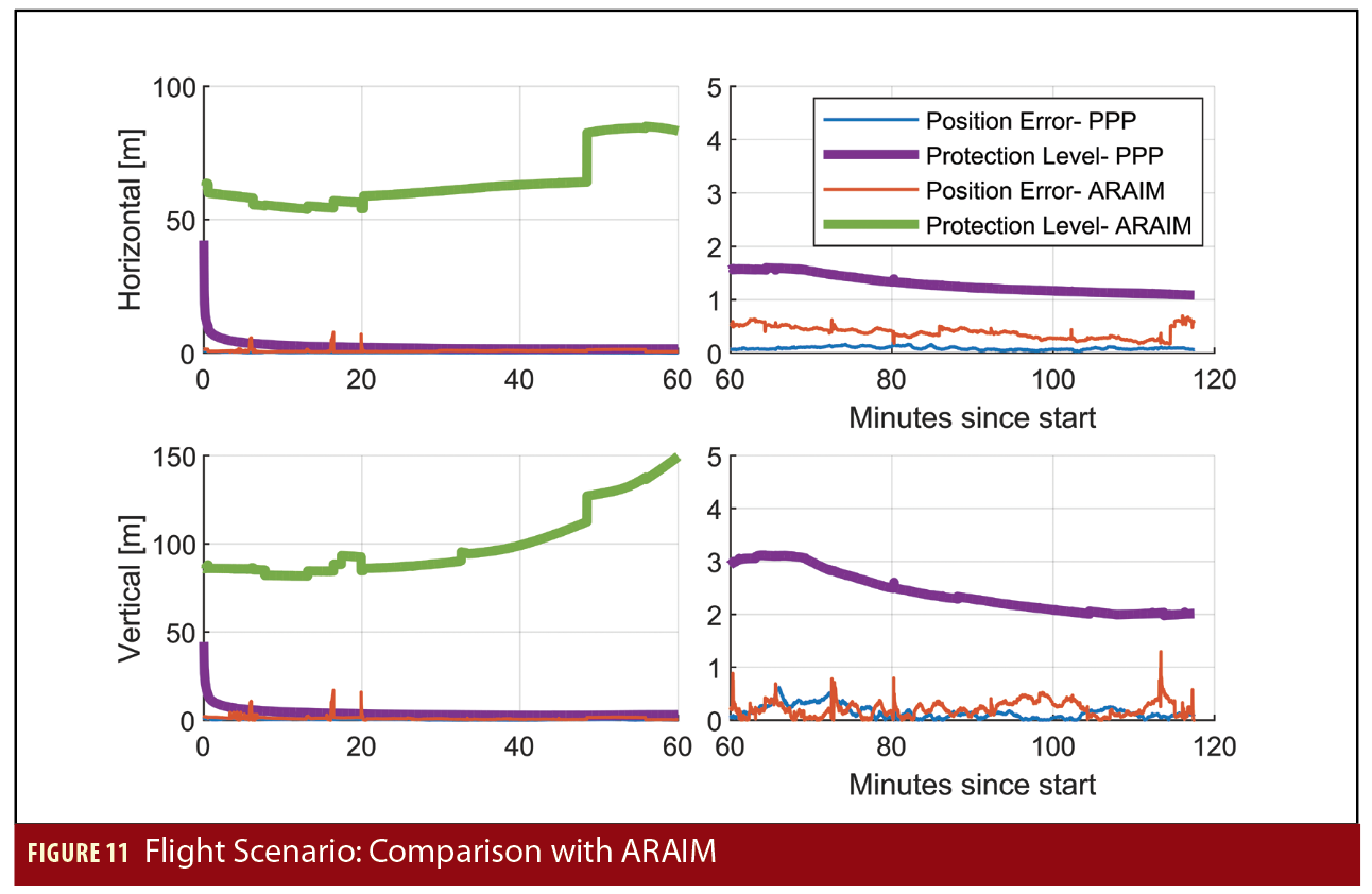
The final scenario compares the performance of PPP-based solution separation with that of Advanced Receiver Autonomous Integrity Monitoring (ARAIM), which the approach outlined in this article is based on but uses multi-GNSS carrier smoothed code in a snapshot solution. This scenario comprises of nearly two hours of flight data from an FAA Global 5000 aircraft. For information on the receiver, see Manufacturers. The truth reference is from Natural Resources Canada’s CSRS-PPP service, which is forwards and backwards processed. Figure 11 shows the protection levels and position errors from the PPP and ARAIM solutions. The ARAIM data here was generated using single frequency GPS and Galileo. The ARAIM horizontal and vertical protection levels are generally greater than 50 and 100 meters, respectively, while the PPP protection levels are under 5 meters after convergence. This approach can offer a significant decrease in protection levels.
Error Statistics
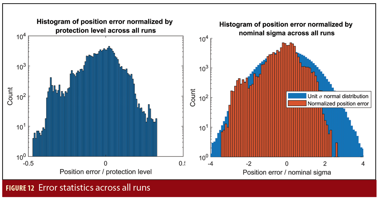
The performance of solution separation techniques relies on the careful characterization of the error models that should then be reflected by the nominal covariance output by the estimator representing the true position error. The plots in Figure 12 show statistics compiled from all of the scenarios previously described. On the right is a histogram of the true position error normalized by the covariance output by the Kalman filter. Under nominal conditions, this should be a unit signal normal distribution, which is shown in the blue in the right figure. The actual normalized position error bound is slightly conservative relative to the ideal. The left plot shows the true position error, this time divided by the instantaneous protection level. The protection level is also conservative, with the normalized error never exceeding 0.5.
Conclusion
RAIM protection level formulas are developed using solution separation, where the formulation consists of a straightforward adaptation of snapshot RAIM to a Kalman filter solution. These formulas are applied to a PPP system, taking care to ensure that the modeling of the PPP solution is such that the true errors match the covariance output by the Kalman filter, and produce meter-level protection levels in static, automotive, and flight scenarios. The results are very promising: Protection levels below 2 meters appear to be achievable, and the computational load is lower than expected.
Manufacturers
The receiver used on top of the building at Stanford University is a survey-grade Trimble NetR9 (Trimble, Sunnyvale, California, USA) and a member of the IGS network. In the Flight vs. ARAIM section of this article, the receiver here is a Trimble BD935 (Trimble, Sunnyvale, California, USA).
In the Open Sky Driving section, the data is from a NovAtel OEM 7500 just outside Calgary International Airport, while the truth positions are generated from a NovAtel OEM729 (NovAtel Inc., Calgary, Alberta).
Acknowledgements
We would like to thank Hexagon Positioning Intelligence for their partnership and for funding this research, Bill Wanner and Mike Gehringer at the FAA William J. Hughes Technical Center for providing the flight data, Stuart Riley at Trimble for lending the receiver used to collect the flight data, and the IGS for the Precise Products used in the PPP corrections.
References
(1) Blanch, J., T. Walter, and P. Enge, “Theoretical Results on the Optimal Detection Statistics for Autonomous Integrity Monitoring,” NAVIGATION, Volume: 64, Issue: 1, 2017
(2) Blanch, J., T. Walter, P. Enge, Y. Lee, B. Pervan, M. Rippl, A. Spletter, and V. Kropp, “Baseline Advanced RAIM User Algorithm and Possible Improvements,” IEEE Transactions on Aerospace and Electronic Systems, Volume: 51, Issue: 1, January 2015
(3) Brenner, M., “Integrated GPS/Inertial Fault Detection Availability,” Proceedings of ION GPS-95, Palm Springs, CA, 1995
(4) de Bakker, P. F. and C. J. M.Tiberius, “Single-Frequency GNSS Positioning for Assisted, Cooperative and Autonomous Driving,” Proceedings of the 30th International Technical Meeting of the Satellite Division of The Institute of Navigation (ION GNSS+ 2017), Portland, OR, September 2017
(5) Gunning, K., J. Blanch, T. Walter, L. de Groot, and L. Norman, “Design and Evaluation of Integrity Algorithms for PPP in Kinematic Applications,” Proceedings of the 31st International Technical Meeting of the Satellite Division of The Institute of Navigation (ION GNSS+ 2018), Miami, FL, September 2018
(6) Kouba, J. and P. Heroux, “Precise Point Positioning Using IGS Orbit and Clock Products,” GPS Solutions, Volume: 5, Issue: 2, 2001
(7) Madrid, P. F. N., L. M. Fernández, M. A. López, M. D. L. Samper,. M. M. R. Merino, “PPP Integrity for Advanced Applications, Including Field Trials with Galileo, Geodetic and Low-Cost Receivers, and a Preliminary Safety Analysis,” Proceedings of the 29th International Technical Meeting of the Satellite Division of The Institute of Navigation (ION GNSS+ 2016), Portland, OR, September 2016
(8) Seepersad, G., J. Aggrey and S. Bisnath, “Do We Need Ambiguity Resolution in Multi-GNSS PPP for Accuracy or Integrity?,” Proceedings of the 30th International Technical Meeting of the Satellite Division of The Institute of Navigation (ION GNSS+ 2017), Portland, OR, September 2017
(9) Working Group C, ARAIM Technical Subgroup, Milestone 3 Report, February 26, 2016; Available at:
• http://www.gps.gov/policy/cooperation/europe/2016/working-group-c/
• http://ec.europa.eu/growth/tools-databases/newsroom/cf/itemdetail.cfm?item_id=8690
Authors
Kaz Gunning is a Ph.D. candidate in the Department of Aeronautics and Astronautics at Stanford University working under the guidance of Dr. Todd Walter. Kaz has previously worked for Booz Allen Hamilton in the GPS Systems Engineering and Integration group doing Modeling and Simulation of OCX and GPS III. His interests are in precise point positioning and integrity.
Juan Blanch is a senior research engineer at Stanford University, where he works on integrity algorithms for Space-based Augmentation Systems and on Receiver Autonomous Integrity Monitoring. A graduate of Ecole Polytechnique in France, he holds an MS in Electrical Engineering and a Ph.D. in Aeronautics and Astronautics from Stanford University. He received the 2004 Institute of Navigation (ION) Parkinson Award for his doctoral dissertation and the 2010 ION Early Achievement Award.
Todd Walter received his Ph.D. in Applied Physics from Stanford University in 1993. He is a Senior Research Engineer in the Department of Aeronautics and Astronautics at Stanford University. His research focuses on implementing high-integrity air navigation systems. He has received the ION Thurlow and Kepler awards. He is also a fellow of the ION and has served as its president.
Lance de Groot holds a B.Sc. and M.Sc. in Geomatics Engineering from the University of Calgary. He joined Hexagon Positioning Intelligence in 2008 and has worked on ground reference receivers for SBAS networks, high precision positioning and relative alignment algorithms for commercial applications and safety critical software for autonomous applications. He is currently a member of Hexagon Positioning Intelligence’s Safety Critical Systems group.
Laura Norman obtained her B.Sc. and M.Sc. in Geomatics Engineering from the University of Calgary. Her research focused on investigating the performance of low-cost consumer grade GNSS receivers for position and trajectory length estimation. Since 2017 she has been a Geomatics Engineer in Hexagon Positioning Intelligence’s Safety Critical Systems Group