In recent years, numerous, relatively inexpensive hardware platforms for conducting scientific research using the software defined radio (SDR) paradigm have become commercially available. The Manufacturers section near the end of this article lists examples of several of these. In turn, this has spurred universities and research groups around the world to adopt this technology for advanced GNSS signals-based research and development.
In recent years, numerous, relatively inexpensive hardware platforms for conducting scientific research using the software defined radio (SDR) paradigm have become commercially available. The Manufacturers section near the end of this article lists examples of several of these. In turn, this has spurred universities and research groups around the world to adopt this technology for advanced GNSS signals-based research and development.
Popular research topics exploiting GNSS SDR receivers include “first look” GNSS signal capture and analysis, interference/spoofing detection and mitigation, GNSS signal authentication by means of nominally present satellite signal distortions (i.e. signal “fingerprinting”), signal quality and deformation monitoring, GNSS bi-static radar and synthetic aperture radar (SAR)-based imaging, multi-platform combined GNSS signal processing, advanced GNSS multipath mitigation, multi-element phased array processing, ultra-tight integration of GNSS with multiple sensors, vector tracking loops and other “holistic” and “open loop” signal tracking approaches, ionospheric research using multi-frequency GNSS observables, and general multi-constellation/multi-frequency GNSS receiver development, prototyping, testing and algorithm validation.
The general approach to carrying out such research involves one or more data collection campaigns followed by mulƒtiple cycles of algorithm development, sampled data processing, and analysis. Realtime processing capability is generally not required at this stage of development. However, to achieve maximum productivity researchers find it highly desirable to have flexibility in algorithm development by way of high-level programming languages and robust user-friendly development environments with extensive built-in math library support and data visualization capabilities. Arguably, within the satellite navigation community, MATLAB has become the de facto standard in this regard.
Many of the afore-mentioned research topics can involve sampled signal data collection at wide bandwidths, high dynamic range, and multiple coherently sampled streams. For example, consider a wideband GNSS data collection campaign for investigating phased array based interference mitigation techniques using a seven-element, controlled reception pattern antenna (CRPA). In this case, bandwidth, dynamic range, and multiple channels are all in play.
Assuming typical front-end hardware specifications for such an application of 60 megasamples per second, 14-bit samples (extended to two bytes for data transfer) and eight channels (one channel being a separate reference antenna), the data capture rate equals 960 Mbytes/second. Even with lesser requirements, it is not uncommon to return from a collection campaign with multiple hundreds of gigabytes (if not terabytes) of data. Thus, a solution is needed to process such large datasets in a reasonable amount of time.
Today’s general-purpose desktop and laptop computers provide tremendous numerical computation capability at low power and cost. This is made possible with multiple processor cores — each clocking at multiple gigahertz and supporting wide single-instruction-multiple-data (SIMD) instructions. In addition, today’s affordable consumer-grade solid-state drives feature sustained read speeds on the order of 500 megabytes/second. Hence, these machines are good candidates for crunching through large amounts of SDR data. For further discussion about computational workloads, see the sidebar (at the end of this article), “Cost/Benefit Justification for a GNSS SDR Toolbox.”
Unfortunately, the layers of software abstraction built into high-level development environments to facilitate user-friendly coding is one of the main reasons why, in general, these tools cannot take full advantage of the computation capabilities of the platforms they run on. Thankfully, all such tools support extensions to allow users to integrate their own custom libraries written in low-level code. In MATLAB, this extension framework is known as “MATLAB executable” (MEX).
The goal of the work reported in this article is to develop a truly universal GNSS SDR processing toolbox for education and research that could be distributed in the form of a plug-in for high-level algorithm development platforms — specifically MATLAB. The following high-level features were envisioned for the toolbox:
- supports the ability to perform a wide range of cutting-edge GNSS signals-based research topics as described previously
- supports most SDR data file formats and front-end frequency plans
- supports all current and emerging GNSS signal structures and other signals of opportunity
- has a user interface and configuration methodology that is easy to learn and apply to the various research topics described here
- provides as many open-source functional examples as possible, thus shortening the learning curve for both beginners as well as advanced users.
The work described in this article achieves, to a large extent, all of these objectives and, more importantly, builds the framework for the baseband signal-processing layer of a truly universal GNSS SDR architecture. The toolbox has been used successfully to process the following open GNSS signals using live data: GPS L1 C/A, GPS L2C, GPS L5, GLONASS FDMA signals on L1 and L2, Galileo E1 CBOC signals using BOC(1,1), BOC(6,1) and CBOC(6,1,1/11) processing; Galileo E5a and E5b, BeiDou B1, satellite-based augmentation systems (WAAS and EGNOS), and WAAS signals on L5.
The software is currently distributed as a MATLAB toolbox and can be downloaded free of charge for education and research use.
One important note: this toolbox is not a complete GNSS receiver in the sense that it does not output position, navigation, and time (PNT) solutions. However, the processed-signal outputs (available at a one-kilohertz rate) contain all the information needed for subsequent processing of PNT solutions.
Supporting Multiple GNSS SDR File Formats
Most SDR data collection systems store their IF-sampled or baseband-sampled data in binary format. For uninterrupted collections over prolonged intervals, data are sometimes written to multiple small files because such a strategy allows files to be managed more effectively than one file written to a large-capacity volume. For systems that collect SDR data continuously for the purpose of recording rare anomalous signal events, this multi-file collection strategy allows older files to be deleted to make space for new ones, thus extending the availability of past history to the size of the storage array in contrast to the capacity of a memory-based buffer.
In some systems, the GNSS samples may be interlaced with binary data from other sensors such as IMUs, laser scanners or cameras to achieve inherent time synchronization between these sensors. In this case, additional metadata information is needed to extract GNSS samples from the file and, optionally, decode the sensor data.
Currently no standard exists within the PNT community that allows GNSS SDRs to work seamlessly with files written by any SDR data-collection system. This means that the user is forced to set data decoding parameters in an ad hoc manner. When files from a different system are sourced, these parameters and the decoder must be changed manually — a process that is prone to human error.
Part of the effort described in this article aims to address this issue so that files from any data collection system can be seamlessly integrated into any GNSS SDR processing platform. The proposed solution is to pair a metadata file with each binary data file. The metadata file includes all the information needed to integrate the SDR file into the processor and decode its contents.
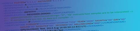
As the format for the metadata file, eXtensible Markup Language (XML) provides a desirable option. All operating systems and application development suites support XML, which is a low-overhead human-readable format, thus providing a straightforward process to integrate it into any data collection system. Figure 1 shows an example of an SDR metadata file written in XML. It contains all of the necessary information to decode the multi-stream samples correctly as well as other information pertaining to the data collection campaign.
The SDR toolbox uses this metadata mechanism to open and decode SDR data files from many data collection systems. When opening a specified SDR file, the reader automatically parses the XML file and imports the metadata into the MATLAB workspace as a structure. For multiple files, the user specifies the name of the first file along with the maximum number of one-millisecond blocks to be processed. This information is used to automatically find and splice the necessary files to fulfill the request.
Supporting a Wide Range of Research Applications
In broad terms, GNSS baseband signal processing can be divided into three stages. The following sections summarize the features required in each of these stages to support a wide range of research applications.
Pre-Correlation Processing. As is well known, correlation losses become negligible for sample quantizations beyond two bits. However, this does not hold true in the presence of interference. In this case, we can use additional dynamic range to perform interference reduction processing prior to correlation. Typical pre-correlation processing includes sample covariance computation (for interference detection and location) and digital filtering and excision techniques applied in the time and/or frequency domains.
The various types of pre-correlation processing that a researcher may want to apply to a GNSS processing application could be supported by including 1) an optimized sample statistics processor, 2) a sample masking processor for blanking interference-dominated samples from being correlated, 3) a configurable time-domain filter implementation (such as Direct-Form II), and 4) a fast Fourier transform (FFT) engine for implementing frequency-domain interference detection and excision techniques.
These processing blocks could be integrated into the sample streams using a software plug-in interface. Since implementations already exist in MATLAB, developing a fully featured pre-correlation processor was considered a lower priority compared to the correlation engine. However, Version 3 of the toolbox does include a sample statistics and noise processor as described in below.
Correlation Processing. Three fundamental techniques exist for sample correlation: time-domain correlation, parallel frequency correlation, and parallel code correlation. The latter two methods provide a large number of correlation outputs corresponding to Doppler frequency offsets or code phases, respectively.
The limited resolution of parallel correlation algorithms and the inability to steer the local replicas that produce them with adequate precision (particularly with respect to code phase) preclude their use in precision signal tracking applications. The parallel code correlation algorithm is most efficient when researchers need a large swath of code correlation space observability such as during signal acquisition. Other uses include correlation space monitoring (also known as delay-Doppler map monitoring) for applications such as spoofer detection.
In any case, a low update rate on the order of one to several seconds is typically sufficient for monitoring applications. As MATLAB already contains optimized FFT implementations to write parallel correlation algorithms, no attempt was made in this version of the toolbox to accelerate FFT-based parallel correlators.
Many of the GNSS SDR research applications described here require several more time-domain correlators than the typical two to five needed for traditional signal tracking. Supporting a given processing algorithm for all current and future GNSS signals can become cumbersome due to their various signal structures.
The ability to instantiate any number of correlators per channel (where each channel can be setup for any GNSS signal structure), and have all these correlators and channels managed with little-to-no user intervention is one of the most desired features of a universal GNSS SDR. This is because it allows the researcher to focus on higher-level algorithm development without having to be concerned with correlator implementation details. Bringing this idea to fruition was one of the major goals and contributions of this effort. The following section describes the architecture of these universal GNSS correlators.
Post-Correlation Processing. Following sample correlation, the data rate is reduced to an easily handled value of one kilohertz. Most of the specialized GNSS signal processing algorithm development occurs in this post-correlation domain. This is also where the strengths of high-level algorithm development tools such as MATLAB shine in terms of a researcher being able to modify scripts and visualize the effects quickly and easily.
An SDR toolbox must feature an interface to and from this domain that is both efficient and intuitive in terms of configuring and controlling the various types of channels and correlators as required by the researcher.
Functional Architecture
This article serves as an introduction to Version 3 of the GNSS SDR toolbox. This version’s functional architecture is significantly different to that of the previous version (v2) that was described in the paper by S. Gunawardena (2013) listed in Additional Resources.
Figure 2 shows the high-level functional block diagram of the GNSS SDR toolbox for MATLAB. Sampled data streams are read from source SDR data files, followed by buffering and decoding into one or more data streams. The streams are fed into two main signal-processing blocks: a stream statistics and noise processor, and a multi-channel ChipShape correlation engine.
To maintain a regular channel architecture that is not specific to any GNSS signal structure, the toolbox uses memory codes exclusively for all pseudorandom noise and masking sequences. These codes are fetched from files and saved in a cache that is accessible to both processing blocks. This code cache is fully configurable by the user such that unused codes can be swapped out for new ones at runtime.
The stream statistics and noise processor computes sample means, variances, and histograms for every one-millisecond block of samples. Sample statistics provide a valuable low-latency “situational awareness” indication of in-band interference. Researchers can use the raw one-millisecond outputs of this processor to prototype a range of interference detection/monitoring algorithms. The toolbox includes commands to disable these computations if not used.
In GNSS receivers, a channel control state machine is typically used to handle the transition from acquisition to steady-state tracking (and subsequent reacquisition to tracking following loss-of-lock events). A low-latency signal-to-noise ratio (SNR) estimate is used as one of the inputs to this controller. Hence, the SNR calculation requires an estimate of noise power, in general for each sample stream.
Some receivers employ a spare channel to compute this noise estimate by correlating with a PRN sequence that is known to be absent in the data. The toolbox implements these noise correlators within the stream processor block. To reduce computation load, noise correlators implement only the real component, and the numerically controlled oscillator (NCO) phase register sizes are also smaller than those used for tracking channels.
As with the statistics processes, each noise correlator can be turned off to improve runtimes. Because these noise correlators can be set to correlate with any of the configured memory codes (including for example, a dedicated random-noise code of any length), the likelihood of significant cross-correlation with in-band signals can be minimized.
Version 2 provided instantiation of any number of correlator points per channel, where each could be connected to one or more universal code generators with independently variable relative code phase delay. Even though this architecture facilitates a wide range of applications, this earlier version repeated the underlying sample-level multiply-accumulate operations when points were placed with less than one-chip separation from each other.
Version 3 eliminates these repeated operations by natively performing ChipShape correlation on an array of points. Ranges of points from this ChipShape output vector can be combined (at the user level) to form any desired points of the traditional triangular correlation function. For binary offset carrier (BOC) signals, the need for a subcarrier replica in the correlation process is also eliminated because the user can apply any subcarrier function as part of the ChipShape-to-triangular conversion step described previously.
Further, by applying chip masking patterns that are specific to the spreading code (combined with long coherent integration), transients of the underlying signal can be observed at high fidelity.
This technique has applications in advanced multipath mitigation, signal quality monitoring and authentication. The paper by S. Gunawardena et alia (2012) listed in Additional Resources provides an overview of ChipShape processing, the concept of chip masking, and its applications in signal quality monitoring.
Figure 3 shows the functional architecture of a Version 3 channel. As with previous versions, the user can instantiate any number of these channels in the toolbox. The main user-configurable channel parameters are shown in red.
The Stream Index parameter selects the input data stream to be processed by a channel. Carrier wipeoff is performed on this selected stream using the replica generated by the carrier NCO — controlled by phase-rate commands updated each millisecond. The carrier-wiped stream is then sent to independent banks of correlators that perform ChipShape correlation for a one-millisecond block of samples. The result is a ChipShape vector for each bank that is transferred to the user space (i.e., MATLAB workspace).
Each ChipShape bank is configured independently by means of three parameters: the number of correlation points per chip NC, the whole number of chips spanning to the early side NE (relative to code NCO integer phase), and the whole number of chips spanning to the late side, NL. Hence, the size of the ChipShape vector is given by NC·(NE + NL + 1), and the spacing between points is given by 1/NC.
As shown in Figure 3, ChipShape processing essentially splits traditional correlation into partial accumulations, where the fractional state of the code NCO determines the array index applicable to the partial accumulation being processed. Splitting the correlation operation in this way maximizes opportunities for these accumulations to be combined in user space to form numerous correlation and/or code discriminator functions depending on the application. Another welcome benefit is that this method reduces the dynamic range required to prevent overflow of these accumulators by a factor of 1/NC compared to a traditional correlator.
Not shown in Figure 3 are the three levels of enable/disable logic featured in the toolbox to improve runtimes: 1) enable/disable entire channels that were instantiated (also disables channel NCOs), 2) enable/disable banks that were instantiated within a channel, and 3) enable/disable individual points within a given bank.
If a ChipShape correlator is implemented as described thus far, the output vector would simply be the differential of a traditional triangular correlation function. Although useful, it does not provide full insight into chip transition edges and their precise zero crossings. The rising, falling, and stationary parts of a GNSS signal’s underlying code sequence can be recovered by correlating with a local replica that corresponds only to these events (e.g., to recover the rising-edge, keep all -1 to +1 chip transitions in the code sequence and set others to zero).
As shown in Figure 3, this functionality is implemented by multiplying the carrier-wiped sample stream with an optional masking sequence. (In actuality the mask bit is used to disable accumulation for that sample.) Each bank is configured independently to point to any code and/or mask sequence stored in the Code Cache shown in Figure 2.
Applying the ChipShape Correlator
The native ChipShape correlator architecture of Version 3 significantly expands possibilities for advanced GNSS signals-based research beyond what was possible with Version 2. Among these are the following examples.
Built-In Acquisition and Rapid-Reacquisition. A dedicated channel can be instantiated for acquisition and/or rapid reacquisition. This channel’s ChipShape vector would span a significantly larger range of integer chip offsets with coarse inter-point spacing (e.g. NC=2 for BPSK, NC=4 for BOC(1,1), and so on). A given PRN can be acquired by pointing to the corresponding memory code and progressively searching for sets of code phase offsets and Doppler frequencies over time.
For reacquisition, the channel’s carrier and code NCOs are set with best estimates of Doppler frequency and codephase, respectively. In this case, ChipShape points corresponding to unnecessary span may be disabled to reduce runtimes. An estimate from the noise processor can be used as the basis for setting up the acquisition detection threshold.
Spoofer Monitoring. A civilian GPS spoofing scenario described in the paper by T. E. Humphreys et alia (Additional Resources) attempts to pull a receiver tracking channel away from the genuine signal’s correlation peak by coercing it to lock on to a stronger peak produced by the spoofer. Even if Doppler offset and codephase are perfect matches to the genuine signal, the superposition of the two would cause significant distortion of the ChipShape function due to the spoofer’s RF transmitter transfer function (which itself is a function of its characteristic analog RF components including modulators, amplifiers, filters and antenna).
A monitor/detector could be implemented using the GNSS SDR toolbox based on a high-resolution ChipShape output computed by an additional bank in each channel. To reduce runtimes (which corresponds to reducing power in a practical application), this bank can be activated at periodic intervals or at the onset of in-band noise power fluctuations (as monitored by sample variance and/or noise correlators), which is a “cheaper” first indicator of possible in-band interference.
Chip Edge–Based Code Tracking for Advanced Multipath Mitigation. As evident from the ChipShape functions shown in the examples section, zero-crossing rising-edge and falling-edge transitions are the highest-frequency components attainable from any received GNSS signal through correlation processing. This is true regardless of signal structure. Hence, code tracking techniques that are primarily based on these transitions stand to produce the best pseudorange accuracy and multipath mitigation performance possible for any receiver of that bandwidth. Researchers can use the highly configurable ChipShape outputs produced by this toolbox as an enabler for researching novel edge-based code tracking techniques for precision GNSS applications.
GNSS Signal Authentication. Variations present in signal transmission payloads of satellites are known to cause subtle signal deformations that are detectable using appropriate processing techniques. Not surprisingly, ChipShape functions are the cornerstone of these techniques. For authentication applications, the deformation caused only by the satellite payload (as a function of nadir angle) must be isolated from nuisance components that include multipath, receiver antenna/front-end transfer function (including any variations due to temperature, vibration, and aging), and ionospheric effects.
Signal-Processing Applications
This section provides two GNSS signal-processing examples that illustrate the configuration and capabilities of the toolbox.
Tracking and Eye Diagram Extraction for BPSK(1) Signals: GPS L1 C/A. For this example, a Version 3 channel was configured with five banks as follows:
- Bank 1: NC=120, NE=NL=1, Code: “GPS C/A PRN,” Mask: “None”
- Bank 2: NC=120, NE=NL=1, Code: “GPS C/A PRN,” Mask: “GPS C/A PP PRN”
- Bank 3: NC=120, NE=NL=1, Code: “GPS C/A PRN,” Mask: “GPS C/A PN PRN”
- Bank 4: NC=120, NE=NL=1, Code: “GPS C/A PRN,” Mask: “GPS C/A NP PRN”
- Bank 5: NC=120, NE=NL=1, Code: “GPS C/A PRN,” Mask: “GPS C/A NN PRN”
where PRN is the C/A code PRN number used and “PP,” “PN,” “NP,” and “NN” correspond to masking codes in which adjacent positive (P) and negative (N) chip events are isolated from the original C/A code. (The distribution includes a utility that generates these and other masking code files from a given PRN code file.)
The GPS L1 C/A signal was pre-acquired using the FFT-based “Quick Acquisition” utility included in the distribution. The latest distribution includes a fully open-source, single channel–tracking script that features a built-in tracking state controller. This state machine was configured to pull-in from acquisition, perform bit synchronization, and settle with the following steady-state tracking loop parameters: 20 milliseconds pre-detection integration time, 18-hertz, third-order phase locked loop (PLL) bandwidth, one-hertz carrier-aided first-order delay locked loop (DLL) bandwidth, and coherent early-minus-late code phase discriminator with early-late correlator spacing of 0.0167 chips.
The final state activates banks 2 thru 5. Then, using the navigation databit sign derived from Bank 1 (i.e., sign[Prompt-Q]) to keep rising, falling, positive, and negative components of the underlying signal together, the one-millisecond ChipShape outputs are coherently combined for approximately 100 seconds. Accompanying figures show the resulting normalized ChipShape outputs.
Figure 4 shows the GPS C/A code eye diagram from a GPS front-end module with approximately four megahertz bandwidth. The effect of narrow front-end bandwidth compared to the results depicted in the following two figures is clearly evident.
Figure 5 and Figure 6 show eye diagrams for GPS Block IIF-6 (SVN67 PRN06) at 78-degree elevation processed from data obtained with the TRIGR GNSS data collection system developed by the Ohio University Avionics Engineering Center. The final-stage IF filters for these two data streams included a transversal surface acoustic wave (SAW) filter with 24-megahertz/3-decibel bandwidth and a lumped element elliptic response filter comprised of a series of coaxial bandpass filters with 3-decibel bandwidth of 18 megahertz.
The bandwidth is sufficiently high in both eye diagrams to observe the 10 cycles of ripple that occurs within a C/A chip. As described in the article by S. Gunawardena et alia (2012b), these oscillations have been determined to be crosstalk from the P(Y) code modulation.
Careful observation of time intervals just prior to a chip transition in Figure 6 reveals a slight buildup of power. This effect, not observable in Figure 5, is primarily due to the finite impulse response-type characteristic of transversal SAW filters as will be reported in detail in a forthcoming presentation by S. Gunawardena et alia (2014) at the ION GNSS+ in September.
Tracking and E1C/E1B Subcarrier Extraction for CBOC(6,1,1/11) Signals: Galileo E1. For this example, a Version 3 channel was configured with four banks as follows:
- Bank 1: NC=120, NE=NL=1, Code: “GAL E1C PRN,” Mask: “None”
- Bank 2: NC=120, NE=NL=1, Code: “GAL E1B PRN,” Mask: “None”
- Bank 3: NC=120, NE=NL=1, Code: “GAL E1C PRN,” Mask: “GAL E1C FF PRN”
- Bank 4: NC=120, NE=NL=1, Code: “GAL E1C PRN,” Mask: “GAL E1B FF PRN”
where “FF” corresponds to masking sequences where adjacent chips with the same sign are isolated from the original spreading code.
Banks 1 and 2 are used for pilot signal tracking and data symbol extraction, respectively. The ChipShape outputs from these banks are correlated with the ideal CBOC subcarrier functions to produce traditional early, prompt, and late correlation points.
Banks 2, 3, and 4 are initially deactivated. After steady-state tracking is reached, the ChipShape outputs from Banks 3 and 4 are coherently integrated for approximately 100 seconds by performing symbol wipeoff using the known overlay symbols and the data symbols derived from the prompt correlator of Bank 2, respectively.
Similar to the GPS C/A code tracking example, the channel state machine was configured to obtain the same steady-state tracking parameters. However, instead of the bit synchronization state used for GPS C/A code, the Galileo E1 tracking demo uses the included overlay code synchronizer.
Figure 7 shows the one-millisecond prompt correlator outputs (pilot and data) from the acquisition pull-in state to just after activation of banks 2–4.
Figure 8 and Figure 9 show the Galileo FM3 E1 CBOC(6,1,1/11) pilot and data component subcarriers as observed from front-end bandwidths of 18 and 24 megahertz, respectively. As to be expected, the multi-level subcarrier functions experience more distortion with the 18-megahertz front-end compared to 24 megahertz. Also notice that for traditional early-minus-late discriminator-based code tracking, zero crossings do not occur at zero codephase due to band-limiting.
Conclusion
This article introduced the GNSS SDR Toolbox for MATLAB (Version 3). This software performs GNSS SDR baseband signal processing using an optimized multi-threaded approach. The main motivation behind the development of this tool was to accelerate offline processing times for large GNSS SDR datasets. The toolbox improves runtimes by at least a factor of 30 compared to equivalent MATLAB-only scripts.
The main feature of Version 3 is a multi-channel universal GNSS ChipShape correlation engine that can be used as the foundation for advanced GNSS receiver development, algorithm design, and prototyping. It can also be used as an educational tool for demonstrating advanced GNSS signal processing techniques.
The Version 3 distribution contains numerous open-source scripts that demonstrate the setup and use of all major features. The toolbox is available free of charge for educational and non-commercial research use. The software and additional resources are available through the author’s blog: <ChameleonChips.com>. Minimum software requirements needed to run the toolbox include Microsoft Windows (32 or 64-bit) and MATLAB version 2007B or above.
Acknowledgment
This article was adapted in part from a presentation given by the author at the ION GNSS+ 2013 conference on September 19, 2013. The views expressed in this article are solely those of the author and not those of any other person, institution, organization, or entity.
Additional Resources
[1] Ettus Research, Universal Software Radio Peripheral (USRP) (accessed July 2014)
[2] Galileo Open Service Signal in Space Interface Control Document (OS SIS ICD), issue 1.1 (accessed August 2013)
[3] Gunawardena, S. (2007), “Development of a Transform-Domain Instrumentation Global Positioning System Receiver for Signal Quality and Anomalous Event Monitoring.” Electronic Dissertation, Ohio University, 2007 (accessed August 2013)
[4] Gunawardena, S. (2013), “A Universal GNSS Software Receiver MATLAB Toolbox for Education and Research,” Proceedings of the 26th International Technical Meeting of The Satellite Division of the Institute of Navigation (ION GNSS+ 2013), pp. 1560-1576, Nashville, Tennessee, USA, September 2013
[5] Gunawardena, S. (2011), and F. van Graas, “Multi-Channel Wideband GPS Anomalous Event Monitor,” Proceedings of the 24th International Technical Meeting of The Satellite Division of the Institute of Navigation (ION GNSS 2011), pp. 1957–1968, Portland, Oregon, USA, September 2011
[6] Gunawardena, S. (2012a), F. van Graas, “High Fidelity Chip Shape Analysis of GNSS Signals using a Wideband Software Receiver,” Proceedings of the 25th International Technical Meeting of The Satellite Division of the Institute of Navigation (ION GNSS 2012), pp. 874-883, Nashville, Tennessee, USA, September 2012
[7] Gunawardena, S. (2012b), and F. van Graas, “Analysis of GPS Pseudorange Natural Biases using a Software Receiver,” Proceedings of the 25th International Technical Meeting of the Satellite Division of the Institute of Navigation (ION GNSS 2012), Nashville, Tennessee, USA, September 2012
[8] Gunawardena, S. (2014), and F. van Graas, “Analysis of GPS-SPS Inter-PRN Pseudorange Biases due to Receiver Front-End Components,” Proceedings of the 27th International Technical Meeting of The Satellite Division of the Institute of Navigation (ION GNSS+ 2014), Tampa, Florida, USA, September 2014
[9] Humphreys, T. E., and B. M. Ledvina, M. L. Psiaki, B. W. O’Hanlon, and P. M. Kintner, Jr., “Assessing the Spoofing Threat: Development of a Portable GPS Civilian Spoofer,” Proceedings of the 21st International Technical Meeting of the Satellite Division of The Institute of Navigation (ION GNSS 2008), Savannah, Georgia, USA, September 2008, pp. 2314-2325
[10] Loctronix Corporation, ASR-2300 MIMO SDR (accessed July 2014)
[11] MathWorks Inc., MATLAB: the language of technical computing (accessed August 2013)
[12] Mathworks Inc., “Introducing MEX-Files,” (accessed July 2014)
[13] Nuand, bladeRF Software Defined Radio (accessed June 2014)
[14] Ouvry, L., and C. Boulanger and J. R. Lequepeys, “Quantization effects on a DS-CDMA signal,” Spread Spectrum Techniques and Applications, 1998, Proceedings of the 1998 IEEE 5th International Symposium, vol.1, pp. 234,238 vol.1, 2-4 September 2–4, 1998
[15] Sparkfun Electronics, SiGe GN3S Sampler v3 (accessed August 2013)
SIDEBAR: Cost/Benefit Justification for a GNSS SDR Toolbox
For GNSS SDR, the most numerically intensive computations involve correlation of hundreds of millions of signed integer samples for each second of processing. However, these samples are typically less than one byte. Through some straightforward pre-processing steps to reduce dynamic range, the result of correlation over a one-millisecond interval can usually be made to fit within 16-bit signed integers with negligible loss of performance.
Hence, these structurally regular fixed-point computations can be parallelized by factors of 8 or 16 using 128-bit and 256-bit wide Streaming SIMD Extensions (SSE) or Advanced Vector Extensions (AVX), respectively. (AVX has been supported in all x86 processors shipping since 2011.) Further parallelization over the available number of logical processors (up to 8 in most consumer PCs) can yield up to 128x theoretical performance improvement compared to un-optimized code.
Such optimizations require the correlation algorithm to be partitioned so that subsets of the computations can be performed independently in each processor. This type of “fine-grained” architecting of an algorithm to exploit the feature set of a particular generation of processors to the maximum extent possible is best done by human programmers as opposed to optimizing compilers.
Because sample correlation is such a critical component of any GNSS SDR and the algorithm essentially does not change significantly with sampling rate or GNSS signal structure, the cost of low-level optimization can be justified by considering the subsequent time savings that can be gained. This is especially true if the correlation engine can be architected such that it supports a wide range of applications and use cases.


