
A comprehensive look at various concepts related to CDF-overbounding, and a methodology for creating protection volumes that contain positioning errors with a high level of confidence.
SÉBASTIEN TRILLES, ODILE MALIET, JULIE ANTIC, KIN MIMOUNI, THALES ALENIA SPACE, FRANCE
In a broad sense, the notion of integrity refers to the level of confidence one can have in data obtained from a calculation result. In positioning systems, integrity is a measure of the trustworthiness a user can place in a position estimate. Geolocation would be perfect if measurements were error-free, but this is never the case as all device measurements inherently contain errors and noise. Hence, a discrepancy between the calculated position and the true (but unknown) one always exists. As errors and noise contains stochastic part, integrity is fundamentally grounded in probabilistic theory.
Mathematically expressed, integrity is equivalent to assigning a probability of the estimate being outside a defined confidence interval (protection level). The integrity of a positioning system is compromised when anomalies occur, leading to unexpected positioning errors beyond the operational protection level. These anomalies could persist for more than a few seconds within a specific time interval (T). In such cases, the integrity risk (IR) is defined as the probability the true position remains outside the protection level for a duration exceeding T.
For instance, in precision approach operations in aviation, the Standards And Recommended Practices (SARPs) set the IR at 2×10⁻⁷ per approach (150s) and the specific time interval to T=6s. The computation of Protection Level (PL) consists of scaling position error variance to the integrity requirement using K-factors. The K-factors are derived from statistical laws and are critical for ensuring the system’s integrity in various operational conditions, taking into account the errors’ time-correlation [9] [10].
In practical applications, positioning is accomplished using measurements with well-known residual error structure and statistical distributions. Position and time errors are determined by linearly combining the residual errors of the measurements. The process starts with the GNSS navigation solution involving the estimation of a position-time correction x as a solution to the measurement equations linearized around a given position-time priori: WGx=Wb+ε, where G is a m×4 matrix with m the number of line of sight, ε is the measurement noises vector, W is a weight matrix and b is the residual measurements vector. The noises ε are assumed to follow a Normal centered law.
The so called design matrix G is defined as the matrix of partial derivatives of the measurement equations with respect to the parameters of position and time. The partial derivative of the pseudo range with respect to the position correction is obtained from the partial derivatives of the geometric distance D=||Xs-Xr || between satellite position Xs and (unknown) receiver position Xr. Re-writing the geometric distance as D=urs∙(Xs-Xr), the partial derivative of with respect to the positions is the unit vector of the line of sight–urs from receiver to satellite.
The weights per line of sight are built using different model variances related to various contributor to measurement errors: residual system errors (orbit and clock), propagation errors (ionosphere and troposphere), and local errors (multipath, thermal noise and interference). The maximum likelihood method provides the estimate =Sb, where S=(Gt W G)-1Gt W is the 4×m sensitivity matrix expressed in the east (E), north (N), up (U) local frame and time.
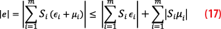
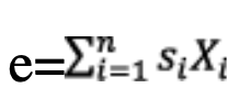
The estimation positioning error e is given by
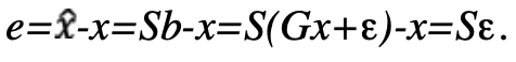
The first three row components of S, respectively sE,i, sN,i and sU,i correspond to the partial derivatives of position errors with respect to the east, north and up directions in relation to the measurement errors of the i-th satellite. The sensitivity matrix linearly projects the unmodeled residual measurement errors εi in a given direction.
For east direction:
for north:
and for up:
This process establishes a straightforward mathematical transfer that enables the projection of residual errors from the measurement domain to the position domain. Focusing on measurement domain, we seek sufficient properties regarding measurement errors distribution that ensure integrity in the domain of positions. These properties define integrity at the measurement level. If these properties are respected, integrity in the domain of positions is ensured, referred to as the transfer of integrity from the measurement domain to the position domain.
This article provides a comprehensive overview of the various concepts related to CDF overbounding. It aims to articulate each concept within a common framework, delineate their ranges and limitations, and ultimately present a methodology for creating protection volumes that reliably contain positioning errors with a high level of confidence.
MOPS Integrity Concept
Initially, integrity concept was developed for aeronautical users and standardized by the Minimum Operational Performance Standards (MOPS) document [1] and is defined at position level. This standard deals with integrity parameters broadcasted by SBAS regarding ionosphere, orbit and clock corrections. In this aspect, MOPS considers the individual measurement error contributors as independent, making it possible to sum up all model variances in unique one σi2 per line of sight. The weight matrix is defined as diagonal W=diag(w1,…,wm) where wi=1⁄σi2).
Therefore, the measurement errors are assumed of white noise type, so their distributions have a zero expectation E[ε]=0, which implies the expectation of the identification error is also zero: E[e]=SE[ε]=0.
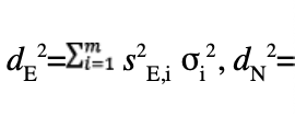
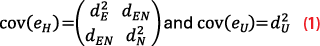
The covariance of the error is: cov(e)=E[(e-E[e]) (e-E[e])t]=E[eet]SE[εεt] St=Scov(ε)St. Therefore, the minimum covariance is reached by taking cov(ε)=W-1, thus cov(e)=SW-1St=(Gt WG)-1. This refers to a four-dimensional symmetric positive-definite matrix whose are linear combinations of the measurement variances, as for instance:
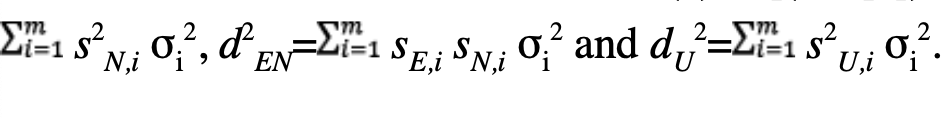
The positioning error structure is then separated into horizontal errors eH and vertical errors eU, which amounts to considering the following extracted submatrices:
The MOPS specify the integrity risk IR as the maximum allowable probability for the navigation position error to exceed the alarm limit without the system alerting the user within the alert time. In the case of a standardized Normal distribution, such as N(0,1), the K-factor depends on the risk IR:
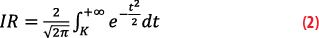
By making the change of variables t=√2u in Equation 2, we obtain an expression that depends on the complementary error function erfc:
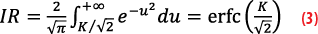
and after inversion in Equation 3, we get the expression of the usual Gaussian K-factor:

Application to protection volumes: The MOPS standard define the vertical protection volume as:

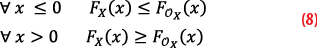
Where the K-factor inflates the standard deviation dU at a level compatible with integrity requirements. Because a linear combination of Gaussian-distributed vector is Gaussian-distributed, the residual position errors follow a Normal law. If ΦeU denotes the cumulative distribution function (CDF) of this Normal law, defined by ΦeU(x)=P(eU≤x), we then have:

Equation 6 indicates that the absolute value of the error eU is bounded by the confidence interval VPL defined in Equation 5 at the probability (1-IR).
The integrity MOPS concept does not mention any overbounding approach. It does not provide information regarding the shape of empirical residual errors distribution. It only mentions [1] the necessity from SBAS to broadcast two parameters, the first one being the variance of Normal distributions associated with the user differential range error for a satellite after application of corrections, and the second one associated with residual ionosphere vertical error at an ionospheric grid point for an L1 signal. The term “associated” as used by MOPS leaves room for several possible interpretations.
In fact, these definitions may give the impression that these Normal distributions represent the actual errors distribution. This interpretation has already been mentioned by several authors [5]. As a consequence, based on the stability of independent Normal distributions through linear combination, the position errors distribution is also represented by a Normal distribution. Unfortunately, the actual range errors are generally not Normal, especially in the tails.
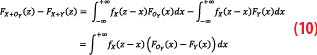
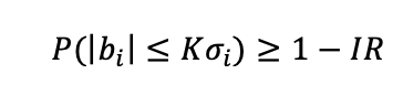
In that context, it could be tempting to check integrity at the pseudorange level by making sure that, for all lines of sight i, the Normal distribution with standard deviation σi is conservative at the quantile equals to the integrity risk IR:

Non-intuitively, this naïve approach is not correct in general conditions. Annex A3 in [1] shows a toy example that satisfies Equation 7 for all lines of sight, and yet is not compliant with the integrity risk IR on position. This example clearly shows integrity transfer from range to position is not obvious and explains the emergence of overbounding concepts.
CDF-Overbounding
The CDF-overbounding concept has been introduced by [2] in the field of aeronautical users. The main idea is to overbound the empirical measurement error distribution, in the field of CDF, by a simpler one allowing to better control the integrity risk mainly in the tails, in the absence of faults. An overbound can be viewed as a statistic distribution that is a regular envelope of the empirical distribution. It is interesting to note the mathematical results presented in [2] were already known to the statistic community [14].
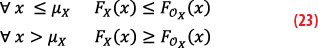
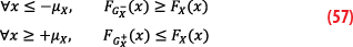
In the following, the CDF of a random variable X is denoted by FX. According to [2], the random variable OX is a CDF-overbound of the random variable X, and we note XOX, if
The binary relationship (8) defines a partial order on the set of distributions. Indeed, the CDF-overbound relation is:
• Reflexive: XX
(every element is related to itself)
• Transitive: if XY and Y
Z then X
Z
(the order is maintained through the chain)
• Antisymmetric: if XY and
YX then X=Y (two elements can’t mutually precede each other; they are considered equal)
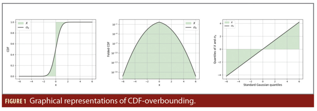
Three graphical representations of CDF-overbounding are provided in Figure 1 for a Gaussian overbound with standard deviation equals to 0.7. The green area represents the domain for the CDF (respectively folded CDF and QQ plot) of X, that satisfies the CDF-overbounding of X by OX. On the left, the CDF of the overbound OX is represented in black. This representation is a direct illustration of the definition. The representation in the middle is based on the folded CDF that equals the CDF before the median and the survival function (1-CDF) after the median. This representation is handy to inspect the overbounding on the left and right tails thanks to the log-scale. The representation on the left is based on the Quantile-Quantile (QQ) plot for X and OX. It permits inspecting both the core and the tails of the distribution.
Introducing the overbounding concept allows the following result:
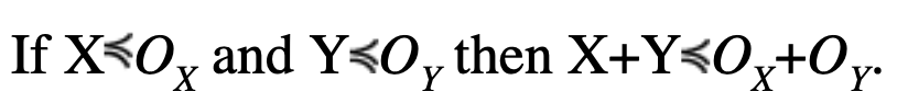
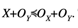
Theorem 1: If X and Y are two centered symmetric and unimodal distributions, and OX and OY their respective overbounds are also symmetric and unimodal. Then for all α, β in , the linear combination αX+βY is CDF-overbounded by αOX+βOY. In short, the overbounding property is stable by linear combination:

If the distribution of each residual measurement error is symmetric, unimodal and can be overbounded by a distribution that is also symmetric and unimodal, then the positioning errors are also overbounded by a known symmetric and unimodal distribution. Under this assumption, integrity in the pseudorange domain implies integrity in the position domain.
Proof:
Proof of stability by addition:
The proof is established in two steps. The first step is to prove that if
The second step is a direct application of the previous statement: if
The sum of two independent symmetric and unimodal variables is itself symmetric and unimodal. The proof is detailed in the Appendix (see online version). This shows all the considered distributions have the right properties to be compared by CDF-overbounding.
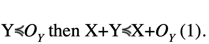
Applying the definition of CDF-overbounding, proving (1) comes down to establishing that:


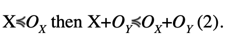
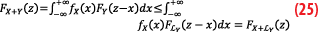
Let us fix z and compute FX+OY(z)–FX+Y(z) using the formula for the CDF of the sum of two independent random variables (the derivation of the formula is recalled in the Appendix):
We now split the integral of Equation 10 into two parts and make the change of variable x to -x for the negative part:
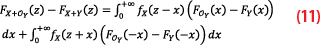
Recalling that by requirement of the CDF-overbounding both Y and OY distributions are symmetrical, which means FY(-x)=1-FY(x) and thus FOY(-x)-FY(-x)=FY(x)-FOY(x). Equation 11 becomes:

By definition of
the right parenthesis of the integrand in Equation 12 is positive for all x. Because X is unimodal and symmetric by assumption, its PDF fX peaks at fX(0) and is decreasing on the positive and negative sides. Thus, the unimodality and symmetry implies that, for all x1 and x2, if |x1|≤|x2| then fX(x1)≥fX(x2).
In our case of interest, if z is negative, we have for all positive x, |z+x|≤|z-x| and so fX(z+x)≥ fX(z-x), which means the left parenthesis of the previous integrand is also positive. We can deduce that

which is precisely the statement (A). On the other hand, if z is positive, |z+x|≥ |z-x| and so fX(z+x)≤fX(z-x) meaning that the integrand is negative and so

This proves (B) completing the proof that, if
and the distributions X, Y, OY are symmetric unimodal, then
By applying the same reasoning, we get that if

and the distributions X, OX, OY are symmetric unimodal, then
This finishes the proof of stability of CDF-overbounding by addition.
Proof of stability by multiplication by a scalar: for all real α,
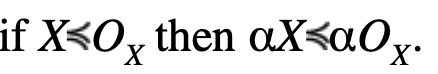
Let X, OX be two symmetric, unimodal random variables such that
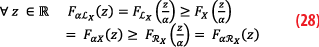
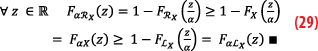
First of all, αX and αOX are also symmetric and unimodal. By symmetry of X and OX, we can restrict ourselves to the case where α is strictly positive. According to the equality FαX(x)=FX(x⁄α) and similarly for OX so the inequalities defining XOX directly translate to αX
αOX.
Application to protection volumes: If X is the distribution of the residual error (symmetric and unimodal by assumption), then a CDF-overbound OX allows us to put a lower bound on the probability of the error to be in a certain interval containing 0. More specifically, for a negative a and positive b, we have: .
Usually, protection volumes are chosen to be symmetric, and thus for positive a,

and so any protection volume computed with the overbounding distribution is a conservative protection volume for the original distribution.
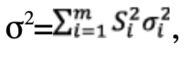
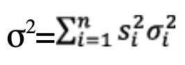
In practice, OX is a Gaussian distribution, chosen for its stability by linear combinations. If in the total error

each error component εi is CDF-overbounded by a Gaussian distribution with standard deviation σi, then the total error e is CDF-overbounded by a Gaussian of standard deviation
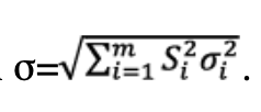
Thus, the usual formula for the protection . Thus, the usual formula for the protection level can be used, with

Case of distributions with bias: The CDF-overbound theorem requires the distributions of error components to be centered. However, the absence of bias in residual measurement errors is never perfectly satisfied because of systematic errors due to troposphere, multipath inter-channel bias, etc.
These errors along the lines of sight are therefore composed of a random part, a noise εi with zero mean, plus an additional bias μi. If these biases were known, they would be integrated into the SBAS corrections, but this is not the case. However, we will assume we know a bound on their absolute values.
The absolute value of the position error along one coordinate is then given by:
We can build the protection volume that covers the suffered errors as follows:
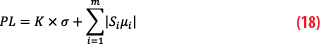
where the factor K is computed according to the error distribution. In the Gaussian case, the multiplicative factor K is calculated using the inverse of the complementary function K=√2erfc-1(IR).
The question of introducing biases as a multiplicative factor of the protection volume calculated with the classic formulation arises. To do this, we introduce the following calculation:
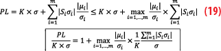
Here, the quantities
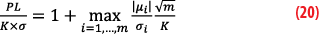
We then find the desired multiplicative factor:
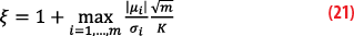
This multiplicative factor ξ makes it possible to inflate the classic volumes of protections (expressed without bias) so as to encompass these residual biases:

This approach allows us to state the following result:
Theorem 1bis: If the distribution of each of the residual measurement errors is symmetric around its median, unimodal and can be overbounded by a Gaussian distribution with the same median (i.e. the mean of the Gaussian is equal to the median of the residual error distribution), then the protection level for the position error can be computed with the usual formula, provided we inflate the K-factor by the multiplicative factor ξ. Under these assumptions, integrity in the pseudorange domain imply integrity in the position domain.
The definition of coverage relative to a median is given by:
The concept of CDF-overbound requires the tails of the overbound cover the tails of the empirical distribution. In the case of a Gaussian overbound, we know the tails of the Gaussian distributions are very light and we will end up finding a quantile (even if it is very large) beyond which the tail of the Gaussian passes below the tail of the empirical distribution. This is why we set in practice a quantile q, beyond the specified integrity risk q>F-1(IR⁄2N), within which, on the interval [-q,q], the overbound property is verified.
Paired Overbounding
This concept was introduced in [3,4] to relax the strong assumptions of CDF-overbounding, namely that the distributions of the residual error components are centered, unimodal and symmetric.
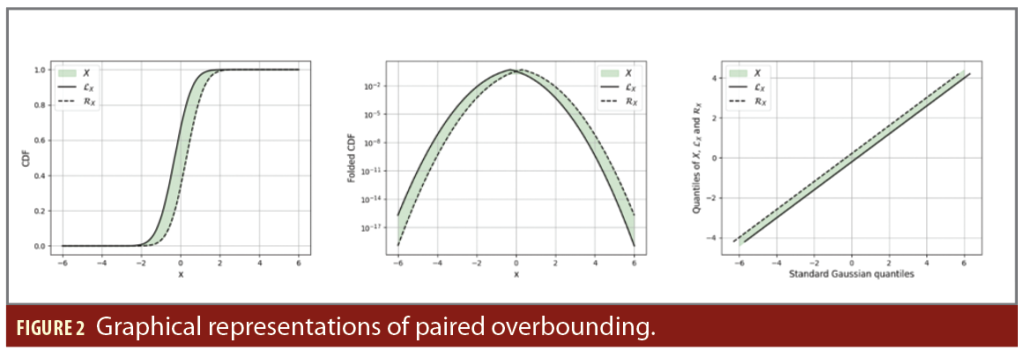
Definition: The random variables LX and RX are a paired overbound of the random variable X, and we note X ⊆ [LX, RX] if
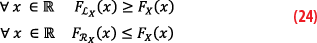
The random variable LX is said to be the left overbound and RX is said to be the right overbound of the random variable X. Figure 2 displays three representations of paired overbounding by two Gaussian distributions with standard deviation 0.7 and bias equals to -/+ 0.3, adopting the same conventions as in Figure 1.
Theorem 2a: For independent random variables X,Y, if X ⊆ [LX,RX] and Y ⊆ [LY,RY] then X+Y ⊆ [LX+LY,RX+RY]. In other words, the pair overbounding concept is stable by convolution. A priori the random variables X,Y and their overbounding pair are arbitrary; no particular assumption is necessary to demonstrate stability by convolution, which is the strength of the concept.
Proof:
We have, using the definition of the left-overbounding:
And so ∀z ε,FX+Y(z)≤FX+LY(z). Repeating the same argument:
Combining the two inequalities of Equations 25 and 26, we get:

The proof of the inverse inequality is established in a similar way without difficulties.
Theorem 2b: If X⊆[LX,RX], then for a positive real α we have αX⊆[αLX,αRX]. However, for a negative real α, we have αX⊆[αRX,αLX]. If we further require that the over-bounding pair is symmetric, meaning that LX=-RX, we can write the result as follows: for all α, if X⊆[-RX,RX], then αX⊆[–|α|RX,|α|RX].
Proof:
We have for positive α:
On the other hand, for a negative α, we have:
These theorems show the stability of linear combinations is satisfied with any pair of overbounds (possibility asymmetric or multi-modal) but only with positive coefficients. Unfortunately, this property is not sufficient to guarantee the integrity transfer from range to positioning domain (because the geometry coefficients are signed). The following Theorem permits to guarantee the stability of any linear combinations (with positive or negative coefficients) by adding a condition on the pair of overbounds that is LX=–RX.
Theorem 2c: If X⊆[–RX,RX] and Y⊆
[–RY,RY] then ∀(α,β)∈2, αX+βY⊆
[–|α|RX–|β|RY,|α|RX+|β|RY]. If the distribution of each of the residual measurement errors is paired-overbounded by a symmetric pair, then the position errors are also paired-overbounded by a known pair. Under these conditions, integrity in the pseudorange domain imply integrity in the position domain.
This approach is useful for taking residual biases into acount. Consider a given line of sight and a contributor X to the residual errors on this line of sight. This contributor presents a residual bias for which a known bound is μ.
We construct a bounding of distribution X by two Normal laws with standard deviation σ, the left bound biased by -μ and the right bound biased by +μ, which form a symmetric pair:
If we collect all the lines of sight and each contributor to the measurement errors paired-overbounded, then the convolution property implies that the position error is also a paired-overbounded distribution with a variance and a bias given respectively by
The limiting aspect is the search for left and right bounds can bring conservatism in practice, knowing these boundaries must frame the entire empirical distribution.
Application to protection volumes: The pair overbounding X⊆[LX,RX] allows us to put a lower bound on the probability to be in a certain interval: for any a,b with a<b, we have:

In the case of an overbounding pair by two Gaussians of mean ±μ and variance σ2, we have for a symmetric protection level:

and so the integrity condition P(X∈
[-PL,PL])≥1-IR can be ensured for

If in the total error
each error component εi is pair-overbounded by two Gaussian distribution with standard deviation σi and mean ±μ, then by the stability by linear combinations, the total error e is pair-overbounded by two Gaussians of standard deviation σ= and mean μ=
. Thus, the formula for the protection level is identical to the formula in the previous section, but with different hypothesis on the original distributions.
Core-Tail Overbounding
In general, the empirical distribution of interest is obtained by collecting large volumes of data. This is sufficient to accurately represent the core of the distribution but there is always a point where the tail remains unknown because the collected samples are always finite. Therefore, how can we ensure the constructed overbounding distribution remains correct for the entire underlying distribution?
Furthermore, if the tail of the underlying distribution is known analytically or with good numerical precision, the overbounding theorems presented impose a condition on the entire distribution. When using Gaussian overbounds, which have very light tails, this can lead to excessive conservatism, for example to absorb some mass far in the tail, or can be mathematically impossible if the analytic expression of the underlying distribution falls slower than a Gaussian.
The strategy presented by [6] is a mean to deal with these two problems. It divides the cumulative distribution function FOX of the overbound distribution into two parts: an explicit core and an implicit tail. The overbounding distribution is a mixture of both, and the value this function takes at a point is equal to the sum of the core cumulative distribution function FOX,c and the tail cumulative distribution function FOX,t, weighted by the probability Pt that the point is in the core or the tail:

The core distribution is explicit, meaning it can be expressed analytically and calculations performed. Most often, it is a Gaussian distribution. As for the tail, which poses the most problems, it is left completely arbitrary: We know it exists, but we do not wish to perform calculations with it. Instead, we will always consider the worst possible tail for the chosen application to constrain the maximum impact of the unknown tail.
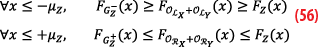
This approach is valid for both CDF-overbounding and paired overbounding. The benefit of this decomposition is to be able to focus on the core overbound, while ensuring the unknown tail of X is defined such that FOX(x) (defined by Equation 34) is an overbound of X, with the following approach of FOX,t as a pseudo CDF:
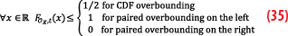
Intuitively, inequality (24) means the worst tail for the CDF-overbounding is a probability weight of 1⁄2 localized at both infinities, whereas the worst tail for a left-overbound is to have all probability concentrated at minus infinity (plus infinity for the right overbound). Formally, the resulting overbounding function FOX(x) is not a CDF (because its total weight is not 1) but as in the excess mass concept, all properties of the corresponding overbounding function remain unchanged.
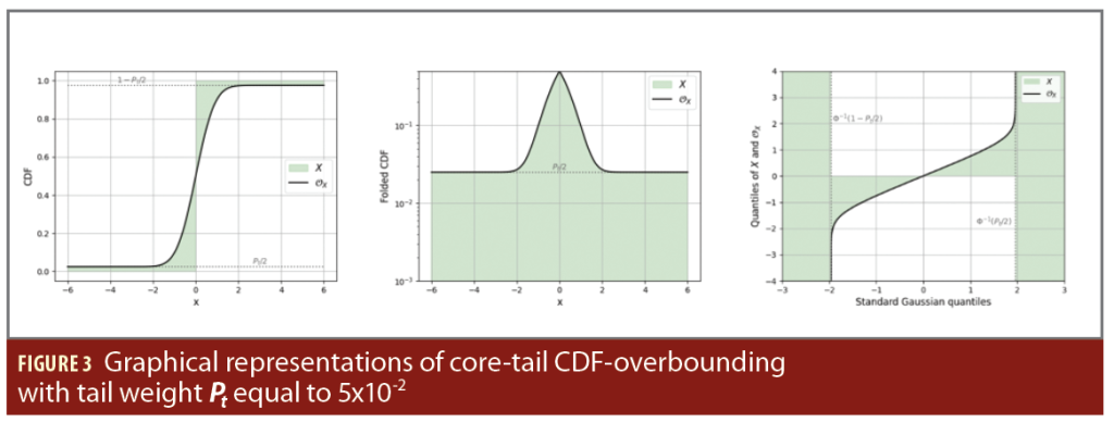
In practice, a CDF-overbound in the core-tail overbounding concept consists of a (symmetric unimodal) function FOX,c and a tail weight Pt such that FOX=(1-Pt) FOX,c+Pt⁄2 (because for CDF-overbounding the tail CDF is always chosen as a constant of value 1⁄2) is a CDF-overbound of the distribution of interest X. In other words, we need FOX,c and Pt such XOX. For pair-overbounding, the left and right bounds are split into core and tail. We need a left and right core overbounding distribution FLX,c and FRX,c and a tail weight Pt such that:

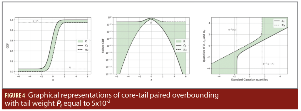
Graphical representations of core-tail overbounding is illustrated with Pt equals to 5×10⁻² in Figure 3 for CDF-overbounding by a Gaussian with standard deviation 0.7, and Figure 4 for paired overbounding by two Gaussian with biais +/- 0.3 and standard deviation 0.7. The green area represents the domain that satisfies the overbounding of X by OX.
Note the core-tail overbounding is a weaker condition than the original overbounding condition, in the sense that any overbounding distribution (CDF or paired) can be seen as the core overbounding distribution with a tail weight Pt, whatever the value of Pt. The downside is the resulting protection volumes will be more conservative for larger tail weight, and can be undefined if the integrity risk is lower than the tail weight. This phenomenon allows for the following result as part of this new paradigm.
Theorem 4: Let X and Y be two random variables that admits a CDF-overbound (central or paired) that can be decomposed into a core part and a tail part with weight Pt,X and Pt,Y. Then the linear combination αX+βY admits a corresponding overbound with the core given by the theorem 1 or 2c, and with core weight (1-Pt,X)×(1-Pt,Y). Under these conditions, integrity in the pseudorange domain imply integrity in the position domain.
Proof:
We will first consider the framework of the central CDF-overbound and the overbounding of X+Y. Theorem 1 (stability by convolution) gives us X+Y is overbounded by OX+OY (the core-tail overbound remains a centered symmetric and unimodal distributions):

We then inject into inequality (26) the decomposition of the overbounds of the random variables X and Y into core and tail.

By expanding expression (38), we get

On the other hand, the cumulative distribution function of the overbound of the sum is decomposed into core and tail parts:

By identification with Equations 38 and 39 we find that:
1-PO,t=(1-Pt,X)(1-Pt,Y), which gives the weight of the core,
FOX+OY,c=FOX,c*fOY,c, so the core of the sum is the convolution of the cores of each distribution,
The rest of the expression is considered as the tail and its explicit expression is not needed.
The last step is to prove by replacing the implicit tail part by the constant 1⁄2, we still have a CDF-overbounding of the sum. For x≤0, the three terms FOX,t*fOY,c(x), FOX,c*fOY,t (x), FOX,t*fOY,t (x) are smaller than 1⁄2 because each one is a symmetric CDF. Thus, for negative x, FOX*fOY(x)≤(1-PO,t)×FOX+OY,c+PO,t⁄2. On the positive side, the equations are reversed, and we get a CDF-overbound of the sum by considering only the core part of the two distributions. We can replace the tail part by its generic value.
The multiplication by a scalar is treated as in Theorem 1 and does not change the weight of the core or tail.
In the pair overbounding case, the resulting pair is symmetric if the core overbounding pair is symmetric, so formula of theorem 2c holds as long as each individual overbounding pair has the same core and tail weights for the left and right overbounding pair. The proof is very similar to the CDF-overbounding case.
The core-tail overbounding concepts allows us to manipulate a weaker form of CDF or paired-overbounding. It is weaker because the inequalities are not required on the entire CDF but only on the core part. The properties of stability by linear combination of the CDF and paired-overbounding are maintained but at the price of a small “contamination” of the tail for each added term. For each addition, the tail weight grows. An upper bound on the weight of the tail can easily be derived as follows: In the case where all weights are equal with tail weight Pt, we have PO,t=1-(1-Pt )2<2Pt, and by recurrence on n sources of errors, we have PO,t<nPt.
Application to protection volumes: The protection volume formulas are identical to the CDF or paired-overbounding cases, with the replacement of the overbounding distribution by the core plus tail part. If we are working with Gaussian distributions, the properties of stability by linear combination allows us to use the same formulas by changing only the value of the K-factor, which now depends on the weight of the tail distribution. The compatible quantile K of a given integrity risk IR in the position domain is calculated by considering the CDF of the overbounding function and inverting it. The Gaussian K-factor changes for the CDF-overbound to:
For a protection volume to be calculable with the K-factor, it is necessary that IR-PO,t>0 and thus that PO,t<IR. Otherwise, the knowledge of the core distribution is not sufficient to build a suitable protection volume and the protection level goes to infinity, and gives no information in practice.
For the paired CDF-overbound the K-factor changes to:
Note the weight of the tail depends on the number of error contributors. If each error has an overbound tail weight Pt<<1, then the full error overbound has tail weight nPt. This means the density of the tail distribution of each measurement error must be at least n times lower than the selected integrity risk for the position domain. In case this condition is not met, the protection volume is undefined (infinite) because the knowledge of the core distribution is not sufficient to guarantee a protection level at the given integrity risk.
If we have Pt<<IR, then we can use the usual K-factor formula (4).
The notion of core-tail overbounding is very important theoretically because it justifies the use of overbounding methods when the tail is not fully known, and it justifies the use of Gaussian overbounding even when the tail is heavier than a Gaussian. However, in practice, such conditions on Pt (Pt<IR⁄n or Pt<<IR) are challenging to verify because IR is already very low (usually about 10-7). This requires a fine knowledge of the error distribution to go far in the tail, which means a large experimental sample of values that is quite difficult to achieve. Thus, the core-tail overbounding technique is rarely used, and the assumption that the overbounding is valid up to infinity is often made.
Excess Mass for Paired Overbounding
In practice, constructing pairs of overbounds can artificially increase biases or variances on each of the overbounds to correctly bound the empirical distribution function. While this operation is often necessary, it inevitably leads to conservatism and larger protection levels than needed.
The left bounding distribution must have a heavier tail on the left (on the negative side) than the original error distribution, while at the same time have a lighter tail on the right. Because Gaussian distributions are often used for overbounding, this double condition is difficult to achieve and is often met at the price of very large biases. This specific problem with the pair overbounding technique can be partially resolved by the concept of excess mass overbounding [5] (excess mass CDF method), which considers a distribution mass greater than 1, typically 1+ ε where ε is referred as excess mass.
With such mass, the pseudo CDF is allowed to pass either beyond +1 or below -1. With this flexibility, we only need to ensure the properties of the overbound on one side of the empirical distribution, knowing the other side is no longer constrained. For Gaussian pair-overbounds, this adds a third degree of freedom to the variance and the bias.
Formally, we consider f, a pseudo-PDF that is positive and integrable, but we do not impose that its total probability weight is 1. Instead, we allow a total mass 1+ε larger than one (Equation 43).

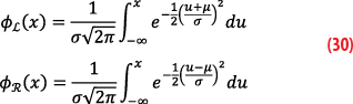
The associated left pseudo-CDF is defined as FL(x)=(1+ε)×F~L(x), where F~L is a regular CDF with total weight equal to 1. This means FL(x) tends to 0 as the variable x approaches negative infinity as a regular CDF, but tends to 1+ε as x approaches infinity, relaxing the overbounding constraint by the left overbounding on the right.
For the right overbound FR(x), the excess mass is applied on the survival function: 1–FR(x)=(1+ε)×(1–F~R(x)), where F~R(x) is a regular CDF, which leads to FR(x)=(1+ε)×F~R(x)-ε. Consequently, the right pseudo-CDF goes to 1 as x approaches infinity like a regular CDF but tends to a negative value when x goes to negative infinity.
With this definition, the concept of pairs of overbounds can be expressed in the same terms and exhibits the same properties, particularly the stability under convolution (the proof can be reproduced identically as it uses only the positivity of the PDF), noting the mass of the sum of random variables is the product of the masses of each variable. Specifically, if the variables X and Y have respectively masses 1+εX and 1+εY, then the sum X+Y has a mass of (1+εX)×(1+εY).
Definition: LX and RX associated to the pseudo-PDF fL and fR define a paired overbound with excess mass ε of the random variable X, and we note X⊆[LX,RX] if
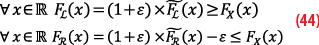
where FL(x) and F~R(x) are regular CDF (with total probability weight equal to 1).
Theorem 3: If X and Y are paired-overbounded with excess mass by a symmetric pair then the linear combinations are also paired-overbounded by a known formula. If X⊆[–RX,RX] and Y⊆[–RY,RY] then ∀(α,β)∈2, αX+βY ⊆[–|α|RX–|β|RY,|α|RX+|β|RY]. (Here –RX is defined as having the pseudo-PDF fR(-x) and the sum and multiplication by a scalar are defined as for regular random variables). The total mass of the overbounding of the linear combination is (1+εX)×(1+εY). Under these conditions, integrity in the pseudorange domain imply integrity in the position domain.
The proof is the same as the equivalent proof for paired-overbounding. With each addition, the total weight of the excess mass overbounding pair grows as it is the product of all masses involved.
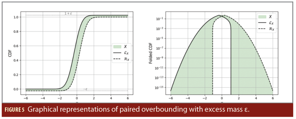
Figure 5 illustrates paired overbounding with excess mass ε equals to 2.5×10⁻². The overbounds are two Gaussian with bias –/+ 0.3 and standard deviation 0.7 and the green area represents the domain that satisfies the overbounding of X by LX on the left and RX on the right. The QQ plot representation is not applicable to excess mass because the overbounds has total weight greater than 1. The allowed green zone is much larger with excess mass than in Figure 2, making the condition easier to verify.
Application to protection volumes: In the case of overbounding by Gaussian pseudo–PDFs, all the convenient addition properties of the Gaussian-distributed vector are maintained. All the formulas derived for the protection volume build with pair-overbounding remain valid, with only a modification in the K-factor. Explicit calculations show the new expression of the K-factor is
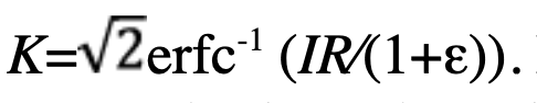
Because the complementary error function erfc is decreasing, we see K increases with ε. Thus, a larger excess mass makes it easier to pair-overbound the distribution, but leads to larger protection volumes.
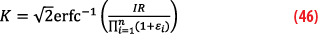
When all the error sources i are paired-overbounded with excess mass by Gaussian distributions of standard deviation σi, bias ±μi and excess mass εi,the calculation of the protection volume remains particularly simple. It is given by

Where
ξ is the multiplicative factor defined by Equation 16 and inflating K-factor defined by Equation 46.
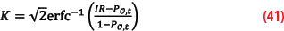
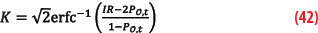
Note the excess mass, as proposed in [5] requires the true tail is Gaussian or lighter to the Gaussian, because the overbound must hold up to infinite. It is interesting to combine the excess mass with core-tail approaches. We propose to include the excess mass only on the core overbound. In this case, we have for each error contributor:

By projecting Equation 47 in position domain, we get:
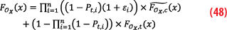
Equation 48 can be arranged as:

By inverting the equation, we get, in Equation 50, the new formulation for K-factor:

Two Steps Overbounding
The objective of the approach proposed in [7] is to mix the two concepts of central CDF-overbound and paired overbound. From the empirical distribution of an unmodelled residual error, the objective is to construct a weaker form of paired overbound by Gaussian distributions (the Gaussian distribution is chosen for computational simplicity).
We start by constructing an intermediate pair-overbound where each bound is unimodal and symmetrical around its mean, but not necessarily Gaussian. We know (Theorem 3) this paired overbound is stable by convolution. We impose the properties of symmetry and unimodality because they are part of the hypotheses of the CDF-overbound. The second step is to find a Gaussian distribution (necessarily symmetrical and unimodal around their mean) where CDF-overbounds the left and right distributions. The assumptions of the CDF-overbound are met and imply these pairs of Gaussians overbounds are stable by convolution.
The result of this method are the two Gaussian variables
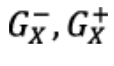
which have the following property:
The resulting properties of the two-step overbounding are weaker than those of the pair-overbounding, but they are sufficient to build a protection volume as follows:

Where K is the usual factor computed with Gaussian distributions (Equation 4).
This protection level is correct because of

The goal is to build a Gaussian two-steps overbound defined by μX, σX that is stable by linear combination, making it possible to perform the overbounding at range level and to build a protection volume at position level.
Theorem 5: If μX, σX define a two-steps overbound of X and μY, σY define a two-steps overbound of Y, then the linear combination Z=αX+βY can be two-steps overbounded by a pair of Gaussians with bias μZ=|α| μX+|β| μY and variance
Under this condition, integrity in the pseudorange domain imply integrity in the position domain.
Proof:
The proof makes extensive use of previous results. Let us start with stability by convolution and consider Z=X+Y. Can we build a two-steps overbound of Z from the two-steps overbounds of X and Y?
We know the intermediate paired overbounding is stable by convolution, and this step requires no particular assumption on the underlying distributions of X and Y:

Then we use that the CDF-overbounding is stable by convolution. This is where the unimodality and symmetry around the median of the intermediate distributions is essential:

Because the CDF-overbounds are Gaussian, we have OLX+OLY~N(μLX+μLY, σ2LX+σ2LY) and similarly for ORX+ORY.
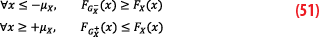
Finally, μZ=μX+μY, we have μZ≥ max (|μLX+μLY|,|μRX+μRY|) and also σ2Z≥ max(σ2LX+σ2LY, σ2RX+σ2RY). Because the tail probability for a Gaussian distribution is an increasing function of the standard deviation and the mean, the previous inequalities ensures the two Gaussian variables
of mean ±μZ and variance σ2Z have the following property:
which is the essential property for the protection level to be correct.
Note these properties on the tails of the distributions are necessary for the protection level formula to be correct but are not in themselves sufficient for a two-steps overbound because they are not stable by convolution. The stability by addition comes from the intermediate paired-overbound constructed in the first step.
The multiplication by a scalar poses no additional difficulties: if Z=αX then Z ⊆ [αLX,αRX] if α if positive (and Z ⊆ [αRX,αLX] for the negative case). In both cases αLXαOLX and αRX
αORX because the considered distributions are unimodal and symmetric around their means. We have αOLX~N(αμLX,α2 σ2LX) and αORX~N(αμRX, α2 σ2RX) and the choice μZ=|α|μX and σZ=α2 σ2X ensures μZ≥max (|αμLX|,|αμRX|) and σ2Z≥max (α2 σ2LX, α2 σ2RX).
The two-steps overbounding construction allows for the transfer of integrity from the measurement domain to the position domain without specific assumptions of symmetry, centering and unimodality of the empirical error distribution by transmitting only two Gaussian parameters per line-of-sight (namely μX and σ2X). This approach is less conservative than the paired overbound by two symmetric Gaussians because the needed property concerns only the left tail
The stability by linear combination is guaranteed by the existence of the intermediate symmetric and unimodal paired-overbound, but the explicit knowledge of the intermediate distribution is not needed for protection volume calculation.
The limiting aspect of the two steps overbounding method is the quality of the final overbound is very dependent on the construction of the first paired overbounds (first step). This step requires a complex optimization algorithm, with one such algorithm described in [7]. Another drawback of the method is it is difficult for a user with knowledge of the original error distribution and the parameters μX and σ2X to verify the received parameters effectively form a correct two-steps overbounding of the error distribution without the information of the algorithm used in the first step.
Wide Sense CDF-Overbounding
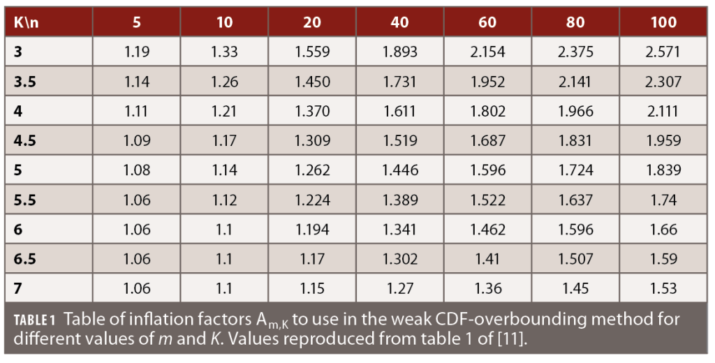
The approach of Weak CDF-over-bounding is introduced in [11]. Similar to the two-step overbound concept, the approach aims at taking advantage of both the CDF-overbounding and pair-overbounding definitions: the simplicity of the first one and the robustness of the second. The main idea is to impose a condition equivalent to CDF-overbounding for biased distribution, but without the assumptions of symmetry and unimodality. When performing linear combinations, the stability of the protection volume formula is lost because of the dropped assumptions. However, it is possible to quantify and bound the worst deviations from the Gaussian distribution and encapsulate them in a suitable inflation factor in the protection volume formula to ensure integrity.
In more precise terms, let X be a distribution (typically the distribution of an error contributor in a GNSS pseudorange measurement) with median b. We do not require X to be unimodal nor symmetric around its median. A weak CDF-overbound is given by a pair of Gaussians with mean ±μX and identical variance σ2 such that μX≥|b| and furthermore:
The condition is identical to the second step of the two-steps overbounding method, but without the first step guaranteeing the stability of the property under linear combinations. If our quantity of interest is given by
where all Xi are individually weakly CDF-overbounded by Gaussian pairs of parameters μi and σi and n being the number of each error source, it is shown in [11] that the weak CDF-overbounding condition is sufficient to build a protection volume for E. The protection level formula is:
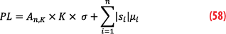
In this formula, K is the usual Gaussian K-factor (σ is the usual Gaussian standard deviation) where
and the new term An,K is an inflation factor that takes into account the weaker assumptions taken in the definition. It quantifies somehow the worst deviations from the Gaussian distribution if each term follows the weak CDF-overbound condition. The inflation factor An,K depends on the value of the K-factor (and the required integrity risk) but also on the number of terms in the linear combination. The factor An,K has no simple analytical formula, but a table of values can be pre-computed and used as such in a given context.
Note the parameter n is the number of independent error contributors and can be larger than the number of satellites in view if there are several error sources for each line-of-sight.
In this method, the properties of CDF-overbounding cannot be used directly because important assumptions on the unknown distribution are not met. However, the conditions of CDF-overbounding by a Gaussian are equivalent to a pair-overbound by two symmetric distributions, the left and right half-Gaussian. Furthermore, the properties of pair-overbounding do not use the assumptions of symmetry and unimodality. One can build a pair-overbound of the final error distribution as linear combinations of half-Gaussians. The last step is to build a pair-overbounding distribution for all coefficients in the linear combinations of half-Gaussians, such that the result is independent of the geometry of the problem. This allows conservative protection volumes to be built for a specific integrity risk. These protection levels are then divided by the usual K-factor and interpreted as an inflation factor An,K integrated in the protection volume formula. Note the factors presented in Table 1 and [11] are upper-bounds and future improvements on the method may reduce the numerical values of the inflation factors and thus of the protection volumes.
The main advantage of weak CDF-overbounding is its simplicity. The condition to verify for weak CDF-overbounding is of the same complexity as usual CDF-overbounding, but fewer assumptions on the underlying distribution are needed. The user only needs to store a pre-computed table of values of inflation factors (computed for the required integrity risk) to use when computing its protection volume. On the other hand, weak CDF-overbounding can lead to large protection volumes if the number of contributors is large and the K-factor is low.
Conclusion
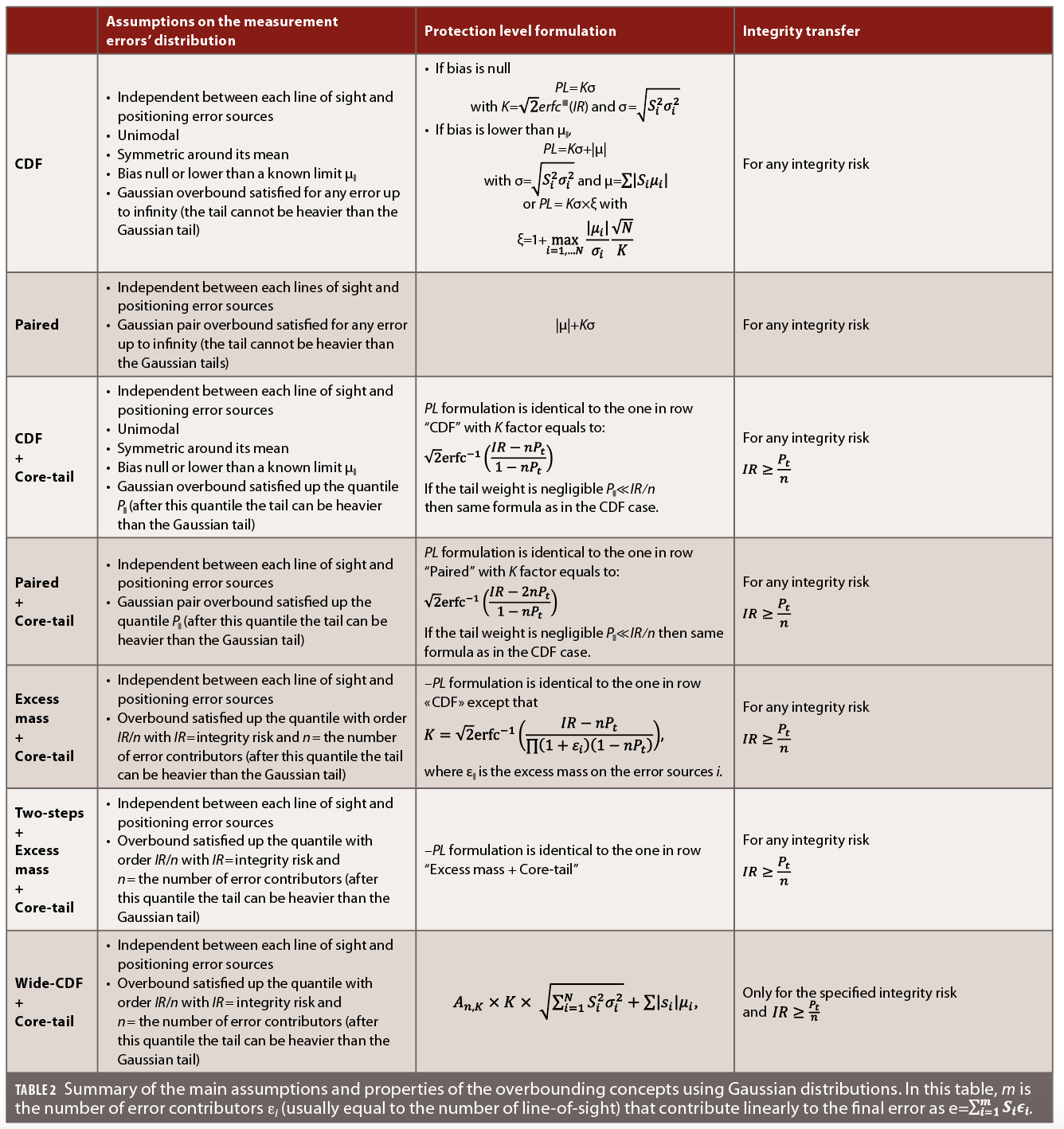
This article shows the overbounding concepts that play a crucial role in demonstrating integrity are neither intuitive nor straightforward. However, the overbounding concepts using Gaussian overbounds are designed to keep the procedure as simple as possible. Indeed, the stability by linear combination of the overbounding properties and of the Gaussian distribution allows the user to manipulate the range errors as if they were Gaussian (by adding their standard deviations in quadrature) and apply the protection volume formula that mostly differ by the K-factor. From the integrity system point of view, the advantage is to focus on monitoring range error distribution and to send few parameters to the user, allowing for the construction of correct protection volumes.
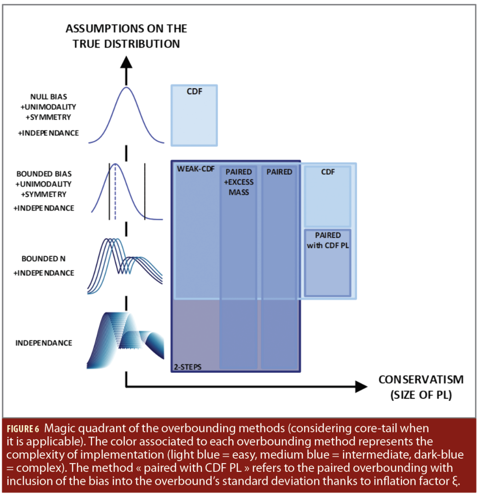
Table 2 summarizes the main assumptions and implications of the different concepts applied to Gaussian overbounds.
Despite extensive work on the subject, several open points remain on overbounding.
First of all, all the studied concepts consider independence between all contributions to the positioning errors, and consequently between line of sights (Table 1). In practice, a correlation between the lines of sight could be caused by the troposphere residual errors, multipath or ODTS algorithm. [12] introduced a Power Spectral Density (PSD) overbounding concept that can guarantee integrity transfer of correlated Gaussian errors (with unknown and arbitrary correlation pattern), using a Gauss-Markov processes that overbound the PSD. To our knowledge, this concept is not used for single point positioning but is key for the integrity demonstration for Kalman filter. Generalization of this concept to non-Gaussian distributions will be a key step both for single point positioning and Kalman filtering.
Secondly, the concepts of overbounding presented are adapted to one dimensional quantities only. For example, the protection level formulas should be applied direction by direction for the positioning solution. A theory of overbounding multidimensional distributions is missing to, for example, build a protection volume for the norm of the horizontal positioning error. One difficulty of such a theory is the norm of a vector is not a linear combination of its components, and thus all the properties presented do not apply to this problem [13].
Last, the practical evaluation of overbounding remains a challenge because it involves estimating quantiles with low probability. This requires collecting and analyzing huge quantities of experimental data, which is costly, cumbersome and generally unrealistic. A promising alternative could be to extrapolate the tails of the distributions beyond the available data based on extreme value theory.
Appendix
CDF OF THE SUM OF TWO INDEPENDENT RANDOM VARIABLES
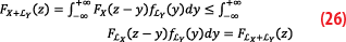
We start by formulating the expression for the CDF of the sum X+Y. By definition of the CDF, F_(X+Y) (z)=P(X+Y≤z). The probability P(X+Y≤z) is obtained by integrating the join density function f_(X,Y) (x,y) of the couple of random variables (X,Y) on the set of x,y respecting the inequality x+y≤z or equivalently y≤z-x. As the random variables X and Y are independent, the joint PDF is the product of the individual PDFs:

The PDF of the sum of the two independent variables X and Y is obtained by making, in Equation 59, the change of variable y=v-x, interchanging the order of integration, and derivating the CDF with respect to z:

Thus, the density f_(X+Y) appear as the classic convolution product Equation 61 of the densities, noted as f_(X+Y)=f_X*f_Y:

The CDF of the sum of the two variables X and Y is obtained by recognizing in Equation 59 the CDF of the random variable Y:

Injecting F_Y (z-x) given by Equation 62 in the expression of F_(X+Y) (z) in Equation 59, we then get:

By making the integral of the joint density function respecting now the inequality x≤z-y in Equation 59, it comes:

Therefore, the CDF of the sum of the two variables X and Y is the convolution of the CDF of the one with the PDF on the other indifferently:

SUM OF TWO SYMMETRIC UNIMODAL RANDOM VARIABLES
In this section, we want to prove the following: if X and Y are two independent, symmetric and unimodal random variables, then their sum X+Y is also symmetric and unimodal [8].
Let f_X, f_Y, be the PDFs of X and Y and f_(X+Y)=f_X*f_Y the PDF of X+Y. Then f_(X+Y) is symmetric because, for all x∈R:

In this manipulation, we have used the symmetry of f_X and f_Y and the change of variable t→-t.
Let us now fix two reals 0≤a≤b and prove that f_(X+Y) (a)≥f_(X+Y) (b). We have from the ordering of a and b that for all x, |x-a|≥|x-b| if x≥((a+b))⁄2 and |x-a|≤|x-b| if x≤((a+b))⁄2. From the unimodality and symmetry of Y, this implies that f_Y (x-a)≤f_Y (x-b) if x≥((a+b))⁄2 and the contrary if x≤((a+b))⁄2. Similarly, we have, for x≥((a+b))⁄2, |x|≥|x-a-b| and so f_X (x)≤f_X (x-a-b) and also, for x≤((a+b))⁄2, f_X (x)≥f_X (x-a-b).
This shows that for all x∈R, we have:

Because both terms are positive for x≤((a+b))⁄2, else both terms are negative.
Integrating the positive product defining by Equation 66 on x, and using the symmetry of f_X,f_Y we get:
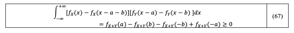
And using the symmetry of f_(X+Y), right side of inequation 67 becomes:

Thus f_(X+Y) is decreasing for positive x, which proves the unimodality of X+Y.
A COUNTER EXAMPLE TO A NAÏVE APPROACH
For a given integrity risk IR and associated Gaussian K-factor, it is tempting to check integrity at the pseudorange level by making sure that for all lines of sight:
However, the following example demonstrates this approach is not sufficient to guarantee the integrity at position level. The reason is this condition tests a certain quantile of the pseudorange error distribution, whereas the stability by linear combinations require criteria to be met across the entire distribution.
Let us use a numerical counterexample. We first take a geometry matrix (here corresponding to 7 GPS satellites above Toulouse on September 3, 2002, 0h00 in ENU frame)
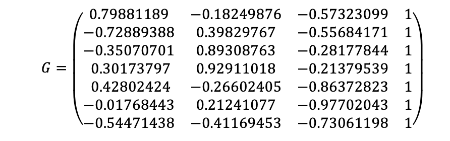
Let us consider the case where all error variances on the pseudorange errors σ_i^2 are equal to 1. Then we build the S matrix as S=(G^T G)^(-1) G^T. The third line of S is

The vertical protection volume VPL has radius given by Equation 69

with K_V=5.33 and σ_V=√(S_(3,i)^2 σ_i^2 )
If the vector of residual errors is
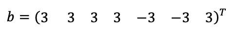
then each line of sight passes the integrity test (meaning that ∀i,b_i<K_V σ_i=5.33), but the vertical error is

which exceeds the protection level radius.
This counter-example does not question the principle of integrity transfers from pseudo distance to position, but the fact that it can be done by the sole definition of confidence intervals in the pseudo distance domain. To establish the equivalence between both realms, the property of overbounding must be verified across the entire distribution, at least up to the desired quantile.
Indeed, if the overbound is applicable for each line of sight, it is extremely improbable to obtain the vector proposed in the example. In addition, if we only know the inequality is satisfied for each line of sight, we have no information about the probability of occurrence of the given vector
in the example, even though it leads to a lack of integrity in the domain of positions.
References
[1] Minimum operational performance standards for Global positioning system/ wide area augmentation system airborne equipment, DO-229, RTCA ed. Washington, DC.
[2] B. DeCleene, Defining pseudorange integrity – Overbounding, In Proc. 13th Int. Techn. Meeting Satellite Div. Inst. Navigat., Salt Lake City, UT, USA, Sep. 2000, pp. 1916–1924.
[3] J. Rife , S. Pullen, B. Pervan, and P. Enge, Paired Overbounding and Application to GPS Augmentation, Proceedings IEEE Position, Location and Navigation Symposium, pp. 439-446, July 2004.
[4] J. Rife, S. Pullen, B. Pervan, and P. Enge, Paired Overbounding for Nonideal LAAS and WAAS Error Distributions, IEEE Trans. Aerosp. Electron. Syst., vol. 42, no. 4, pp. 1386–1395, Oct. 2006.
[5] J. Rife, J. Blanch and T. Walter, Overbounding SBAS and GBAS Error Distributions with Excess-Mass Functions, in Proceedings of the GNSS 2004 Internat. Symp. On GNSS/GPS, Sydney, Australia,6-8, Dec. 2004.
[6] J. Rife, S. Pullen, B. Pervan, Core Overbounding and its Implications for LAAS Integrity, Proceedings of the 17th International Technical Meeting of the Satellite Division of The Institute of Navigation (ION GNSS 2004), Long Beach, CA, Sept. 2004, pp. 2810-2821.
[7] J. Blanch, T. Walter and P. Enge, Gaussian Bounds of Sample Distributions for Integrity Analysis, IEEE Trans. Aerosp. Electron. Syst., vol. 55, no. 4, pp 1806-1815, Aug. 2019.
[8] M. Earnest, link.
[9] J. Antic, O. Maliet, and S. Trilles, “SBAS Protection Levels with Gauss-Markov K-Factors for Any Integrity Target”; NAVIGATION: Journal of the Institute of Navigation September 2023, 70 (3) navi.594
[10] K. Mimouni, O. Maliet, J. Antic, “A simple and robust K-factor computation for GNSS integrity needs”. ION plan, pp 399-407, 2023
[11] Maliet, O., Mimouni, K., Antic, J., & Trilles, S. (2025). Wide-Sense CDF overbounding for GNSS integrity. NAVIGATION: Journal of the Institute of Navigation June 2025, 72 (2) navi.697; link
[12] Langel, S., Crespillo, O. G., & Joerger, M. (2020, April). “A new approach for modeling correlated Gaussian errors using frequency domain overbounding”. In 2020 IEEE/ION Position, Location and Navigation Symposium (PLANS) (pp. 868-876). IEEE.
[13] I. Nikiforov, “From pseudorange overbounding to integrity risk overbounding”, NAVIGATION, Vol 66, Issue 2, Summer 2019, pp 417-439.
[14] Z. W. Birnbaum, “On Random Variables with Comparable Peakedness”, The Annals of Mathematical Statistics, 19 (1), pp 76-81 doi:10.1214/aoms/1177730293
Authors
Julie Antic is a specialist in GNSS integrity algorithms and performances at Thales Alenia Space in Toulouse, France. She holds a Ph.D. in probability and Statistics from Paul Sabatier University, France, as well as an engineering degree in applied Mathematics from INSA in Toulouse, France. Her areas of activity include advanced GNSS augmentation systems for high accuracy and integrity, advanced receiver autonomous integrity monitoring and overbounding concepts.
Odile Maliet graduated from École Polytechnique and received her Ph.D. degree in Macroevolution from École Normale Supérieure (ENS), Paris in 2018. Between 2018 and 2020, she worked as a postdoc on the use of Bayesian techniques on phylogenetics empirical data at ENS, Paris. Since 2021 she has worked on integrity concepts in Advanced Projects at the Performance and Processing Department of Navigation Domain, Thales Alenia Space.
Kin Mimouni graduated from École Polytechnique, Paris, and received his Ph.D. in Theoretical Physics from École Polytechnique Fédérale de Lausanne (EPFL) in 2019. Since 2021 he has worked on GNSS algorithms and integrity concepts, first as a post-doc in the Télécommunications Spatiales et Aéronautiques (TéSA) laboratory in Toulouse, and since 2023 as an engineer in Advanced Projects at the Performance and Processing Department of Navigation Domain France, Thales Alenia Space.
Sébastien Trilles is an expert in orbitography and integrity algorithms at Thales Alenia Space in Toulouse, France. He holds a Ph.D. in Pure Mathematics from the Paul Sabatier University and an advanced master’s degree in Space Technology from ISAE-Supaero. He heads the Performance and Processing Department where high precise algorithms are designed as orbit determination, clock synchronization, time transfer, reference time generation, integrity and ionosphere modeling algorithms for GNSS systems and augmentation.


