
The methods used to establish traceability of the timing data processed by a GNSS receiver to Coordinated Universal Time (UTC), and the role calibrating the delay in the user’s receiving and processing equipment plays in realizing this traceability.
JUDAH LEVINE, UNIVERSITY OF COLORADO, PASCALE DEFRAIGNE, ROYAL OBSERVATORY OF BELGIUM, ILARIA SESIA, ITALIAN METROLOGY INSTITUTE, GIULIO TAGLIAFERRO, INTERNATIONAL BUREAU OF WEIGHTS AND MEASURES, MICHAEL WOUTERS, NATIONAL MEASUREMENT INSTITUTE
Coordinated Universal Time (UTC) has been recommended as the unique time scale for international reference time stamps and is the basis for civil time in most countries [1]. Time zones, which are established by local administrations, are defined by an offset from UTC. Some applications are required to use time stamps based on UTC either by regulation or by statute [2-4]. There are advantages to the use of time stamps based on UTC, even when it is not required to do so, because this facilitates combining data from multiple sources or when international coordination is important.
Time signals from global navigation satellite systems (GNSS) are widely used as the reference time in many applications, and it is important to understand the requirements that ensure GNSS time stamps are traceable to UTC from both a technical and a regulatory perspective [5]. This article describes how UTC is defined and realized and how a prediction of UTC is included in GNSS data transmissions.
The Definition and Realization of UTC
The UTC time scale is a paper time scale that has no physical realization. It is computed monthly by the International Bureau of Weights and Measures (BIPM) based on data from several hundred atomic clocks located at National Metrology Institutes (NMIs) and other time centers in various countries. Many laboratories operate local ensembles of atomic clocks and use the data from these ensembles to compute and disseminate a local UTC estimate. This local estimate is identified as UTC(k), where k is the acronym for the laboratory. The estimate of UTC computed by the U.S. Naval Observatory (USNO) is UTC(USNO) and the estimate computed by the National Institute of Standards and Technology (NIST) is UTC(NIST).
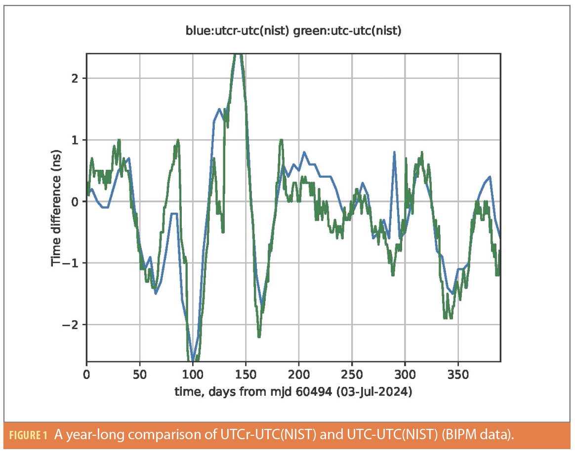
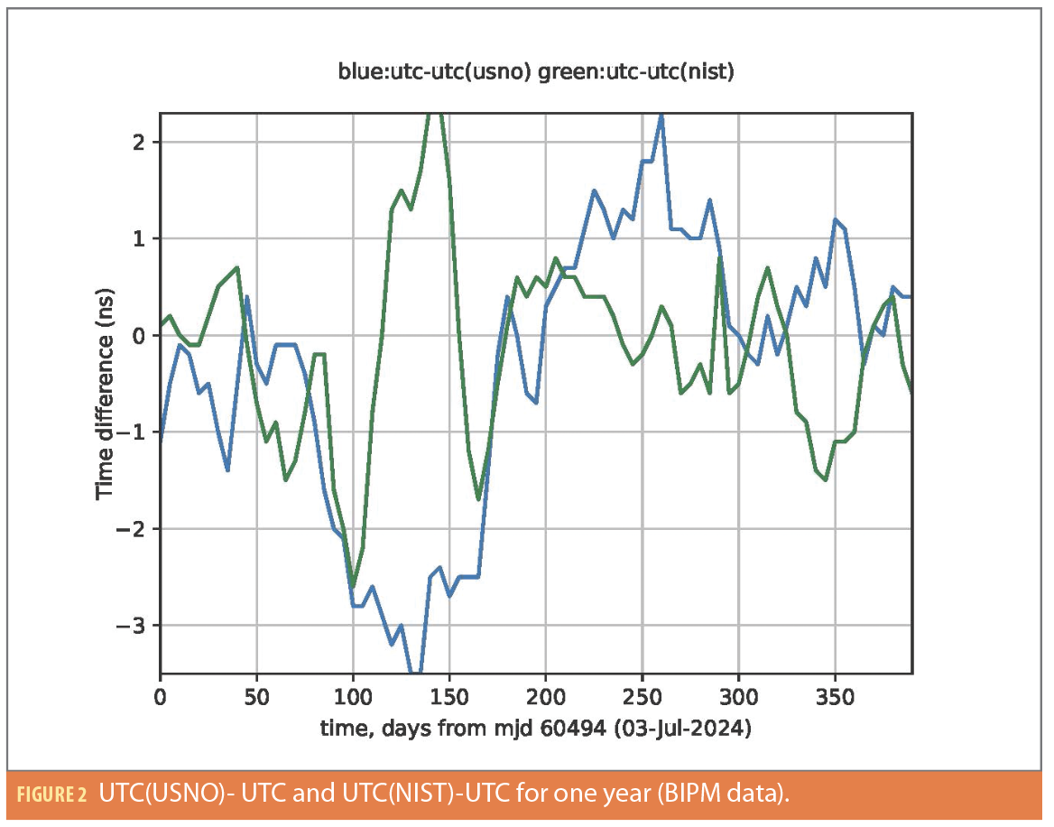
The computation of UTC for any month is published in BIPM Circular T by the tenth day of the following month [6]. This circular tabulates UTC-UTC(k) every five days for every participating laboratory. A rapid version of UTC, called UTCr [7], is also published by the BIPM every Wednesday. It lists daily values of UTCr-UTC(lab) through the previous Sunday. These data are published on the BIPM website and are distributed by email (Figures 1 and 2).
GNSS Time Signals
The system time of a GNSS constellation, GNSS_T, is generated by the ground segment from an ensemble of clocks located on the ground at the control center and tracking stations. It also can include the clocks in the satellites [8-11]. Each satellite in a constellation transmits a prediction of the offset between the time of the clock on the satellite and the system time of the constellation, which is uploaded to the satellites periodically. GNSS constellations also broadcast bUTC_GNSS, a prediction of the difference between GNSS_T and UTC (including a 3-hour offset for the GLONASS system) that is derived from the UTC prediction of timing laboratories. This prediction is transmitted in two parameters: an integer giving number of whole seconds difference between UTC and the GNSS system time, and a fractional part, which specifies the difference modulo 1 s. The first parameter changes only when a leap second is inserted into UTC and not at other times. (The GLONASS constellation uses UTC as the system time so only the fraction is transmitted in the navigation message.)
For the GPS constellation, this prediction is derived from UTC(USNO) maintained at the U.S. Naval Observatory. The GLONASS constellation broadcasts a prediction based on UTC(SU), which is realized at the Russian Metrology Institute of Technical Physics and Radio Engineering (FSUE, VNIFTRI). The Galileo constellation uses a prediction derived from a collaboration of five European National Metrology Institutes. The BeiDou system uses UTC(NTSC) realized at the National Time Service center of China and UTC(NIM) realized at the China National Institute of Metrology. Regional systems also broadcast similar messages. The formats of the respective messages are GNSS-specific and are documented in the respective Interface Control Documents.
The Role of the BIPM
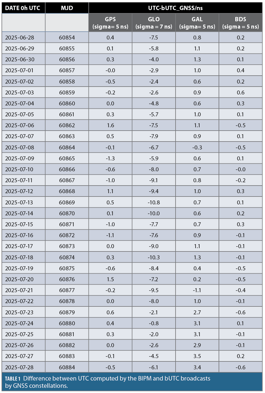
In addition to computing UTC and publishing the differences of UTC-UTC(k), the BIPM evaluates the difference between UTC and the predictions of UTC broadcast by the various GNSS constellations, bUTC_GNSS. These differences are published in Section 4 of BIPM circular T [6]. This section lists the difference in ns between UTC computed by the BIPM and the prediction of UTC transmitted by the GPS, GLONASS, Galileo and BeiDou satellites for every day in the monthly reporting period for that issue of Circular T. Table 1 shows the values from the August 2025 editor of Circular T interpolated from the five-day reporting interval in Circular T to a daily value at 0 UTC [12].
Linking User Equipment to UTC
There are two common configurations that support a link between the user’s time reference and UTC(k) or UTC. In the first configuration, the user has a clock (or an ensemble of clocks) that provides the reference signal for a GNSS timing receiver. The receiver does not discipline the free-running local clock (or ensemble) in the short term, but measures its time with respect to the signal broadcast by the satellites of some constellation. These data are combined with the data in the navigation message to (1) correct for the transit time between the satellite and the receiver, (2) include the offset between the satellite clock and the GNSS system time, and (3) add the prediction of the offset between the system time and UTC.
Most receivers can be configured to implement these calculations in firmware, and the output data gives the difference between the local reference and the broadcast prediction of UTC. The signal from this clock (or clock ensemble) can be used in the user’s application or the application’s clock can be compared to it. The system connected to the GNSS receiver may be completely free-running and not disciplined by the GNSS data; its offset is recorded and used to adjust the downstream data. In some configurations, the time or frequency of the local reference clock is adjusted from time to time so the measured time difference is kept within some administratively defined tolerance. The interval between adjustments depends on this tolerance and on the frequency stability of the local reference, and it can range from minutes for a rubidium-based reference to hours or days for a cesium-based device.
The second configuration, which is much more common, combines a GNSS receiver and an oscillator in a single device. There are many commercial systems that realize this configuration and often provide several outputs (5 MHz, 10 MHz and 1 pps) that are disciplined by the data received from the GNSS constellation. The simpler systems use the code data transmitted on the L1 frequency, but dual-frequency receivers and more sophisticated carrier-phase analyses are possible. The first GNSS disciplined oscillators usually used signals from the GPS constellation, but newer systems can track satellites from more than one constellation simultaneously. The output signal might be based on only the satellites from one constellation at any time or on a combination of the data received from multiple constellations. Either solution can produce significant steps in the output signals, especially in the PPS data, when the reference constellation changes. The details of the disciplining algorithm are often proprietary; the output could be disciplined to GNSS system time or to the prediction of UTC, and traceability to UTC would require the additional adjustment that incorporated the data published in BIPM Circular T. This additional adjustment, based on data from Circular T, may be small enough to ignore in some applications.
The first configuration is more flexible; the measurement process can accept data from multiple sources, including common-view data, and implement more sophisticated post-processing methods. The adjustment process for the local reference clock can be adjusted to meet the requirements of the user’s application. The second configuration, on the other hand, may provide adequate performance in many applications. It is much simpler to operate, and this simplicity may be the deciding factor for many users.
Combining Data from Multiple Constellations
Combining GNSS signals from multiple constellations can significantly improve the timing performance of a user’s receiver, especially in locations with limited visibility of the sky. This approach requires a knowledge of the offsets between different GNSS time scales, which are at the level of a few ns and vary in time. It is possible for a user to solve for the inter-system bias between constellations [13] if enough satellites from both constellations are visible at the same time, but this is not always the case, and the broadcast values must be used [14]. The broadcast of the predicted time difference between each GNSS system time and UTC greatly simplifies the job of combining signals from multiple constellations when only broadcast data are available. The use of UTC as the common reference time scale eliminates the need for maintaining multiple inter-system bias values.
Metrological Traceability
The International Vocabulary of Metrology (VIM) defines traceability as the “property of a measurement result whereby the result can be related to a reference through a documented unbroken chain of calibrations, each contributing to the measurement uncertainty” [15]. The International Telecommunications Union (ITU) [16] and the International Laboratory Accreditation Conference adopted the same definition and refer to the International Organization for Standardization (ISO/IEC) standard 17025 [17].
The signals transmitted by the GNSS constellations can be traceable to UTC. The broadcast signals are linked to UTC through the UTC(k) data of a timing laboratory, and the transmissions are monitored by the BIPM with results published in Circular T. A user can also establish a common-view relationship with a timing laboratory, which can provide a near-real-time estimate of the offset of the user’s timing system with respect to the UTC(k) of that laboratory. In either case, these data are processed by the receiving system at the user’s site, and the calibration and statistical characteristics of this system directly affect the accuracy and stability of the timing data that control the user’s application.
Timing Receiver Calibration
The calibration of the user’s equipment that is required to complete the demonstration of traceability should be performed by a method validated by a National Metrology Institute or a Designated Institute that participates in the Mutual Recognition Agreements (MRA) and have their Calibration and Measurement Capabilities (CMC) published in the Key Comparison Database maintained by the BIPM [18]. The Key Comparison Database maintains the equivalency between different organizations and guarantees the international acceptance of calibrations performed by different agencies that participate in the MRA.
The manufacturer’s published specifications can be the basis for specifying the performance of a stand-alone GNSS receiver or a GNSS receiver and disciplined oscillator combination. These specifications should be based on a calibration of one example of a particular model with some allowance for the variation among devices of the same type. For applications that require only modest accuracy (not greater than about 1 µs) a statement by the manufacturer that the device has been type-approved to that level is sufficient. The transmission delay even through a very long antenna cable is unlikely to invalidate this assumption.
The use of “type approval” may not be adequate for applications that require sub-microsecond accuracy. One method of calibrating a receiving system is to compare the output of the system to a source of UTC(k) by using a time-interval counter to monitor the difference. This method depends on an independent source of UTC(k), which might be provided by a traveling calibrated receiver, by transporting a running clock from the UTC(k) source to the location of the receiver, or by operating the device to be calibrated at a laboratory where a source of UTC(k) is available.
Using a traveling receiver is the best choice because it tests the receiving hardware with the antenna and cables in the environment where it will be used. The BIPM uses this option to calibrate the time-transfer equipment at timing laboratories. Although the traveling receiver is calibrated, it is operated at a location where its position may not be known accurately, and where it may be influenced by multipath effects that are not the same as the effects on the device under test. These considerations are usually not important unless the required accuracy must be better than about 50 ns.
A calibration based on carrying a running clock from the source of UTC(k) to the location of the user’s equipment is feasible if the distance is not too great and the required calibration accuracy is not too high. For example, the GPS receivers at the NIST radio station in Fort Collins, Colorado, are calibrated by carrying a rubidium oscillator from the source of UTC(NIST) in Boulder to Fort Collins, a distance of about 100 km by road. The calibration is repeated by carrying a calibrated GPS receiver between the two locations. The accuracy of either method is estimated to be about 15 ns, and the two methods agree within this uncertainty.
Transporting the device under test to a location where an independent source of UTC(k) is available is usually the most difficult solution. It may be impractical to disconnect the antenna cable at the site, so a different cable must be used for the calibration. The delay through the actual cable can be estimated with a time domain reflectometer, but this method tests the cable with signals that are not the same as signals from real satellites. The impedances at the end-points are also different.
If the system to be calibrated provides the contribution of each satellite in view to the composite output, then the common-view method can be used to calibrate the receiver. (Unfortunately, many disciplined oscillators do not provide these data.) The system to be calibrated measures the difference between the local clock (or clock ensemble) and the system time of the constellation by using the data from each satellite in view. These data are compared, satellite by satellite, with the same measurements made at a location where UTC(k) is available. The common-view difference cancels or attenuates the contributions of the satellite clock and the orbital parameters, which are common to both data sets and cancel in the differences in first order. If the distance between the locations of the user and the UTC(k) laboratory is not too great, the contribution of the ionosphere may also be common to both measurements and cancel in the difference. A multiple-frequency measurement, which can correct for the contribution of the ionosphere, may not offer a significant improvement over a simple L1 comparison in this configuration, because the contribution of the ionosphere will be cancelled or attenuated in the common-view subtraction. The common-view method can operate continuously, and can also monitor the stability of the remote system.
Frequency Calibration
The techniques described for timing calibration can also calibrate the output frequency of the user’s system. A frequency calibration can be easier to realize than a time calibration because the absolute values of the delays in the equipment are not important, only the stability of these delays is. The stability of the output frequency of a quartz oscillator may be degraded by fluctuations in the ambient temperature, and the frequency estimated with a reference based on a rubidium or cesium device may be degraded by changes in the multipath contribution.
Specific Recommendations
The documentation from the manufacturer is the best source of information about a particular device. The following specifications provide general guidance on the methods to establish traceability [19].
1. If the application can accept a fractional frequency uncertainty of 10-8 or greater with an averaging time of one day, or a time uncertainty of 1 µs or greater, then a certificate by the manufacturer that at least one unit of the model satisfies the requirement is adequate to establish traceability at this level. (A receiver used only as the reference for a server that supports NTP, the Network Time Protocol, may not require calibration, because the accuracy and stability of the NTP service is usually limited to not better than about 1 ms by the characteristics of the network connection between the server and the client systems.)
2. If the application requires a fractional frequency uncertainty between 10-8 and 10-10 with an averaging time of one day or a time uncertainty between 100 ns and 1 µs, then the manufacturer should provide a certificate with every unit that satisfies the requirement. The manufacturer could validate the performance of each unit by comparing its output with a calibrated reference unit maintained at the manufacturer’s facility.
3. If the application requires a fractional frequency uncertain of less than 10-10 with an averaging time of one day or a time uncertainty of less than 100 ns, then the calibration can be challenging and should be performed at the user’s facility, if possible.
4. If the application requires a fractional frequency stability of less than 10-12 or a time uncertainty of less than 50 ns, then the calibration should be repeated periodically or the performance of the system should be monitored by common-view or an equivalent technique, which will require a dedicated GNSS timing receiver at the user’s site. The contributions of multipath reflections and the sensitivity of the equipment to fluctuations in the ambient temperature may be important. The impact of multipath reflections can be minimized by locating the antenna so it has an unobstructed view of the sky, and by using a directional “choke ring” antenna, which attenuates signals coming from low elevations. The sensitivity to fluctuations in the ambient temperature may be a problem if the local reference device is a simple quartz oscillator or if a long antenna cable is exposed to direct sunlight.
It is important to maintain documentation that validates the traceability of any system. Configurations that support this capability are particularly useful.
Summary and Conclusion
Applications that use the timing data from GNSS systems often require legal and technical traceability to UTC. Even when traceability is not legally required, maintaining traceability to UTC simplifies combining the data from multiple constellations. The signals transmitted by GNSS systems are monitored by the BIPM and can be made traceable to UTC by the methods discussed. Ensuring the traceability of the timing data in a user application also depends on a calibration of the receiving equipment. The methods for realizing this calibration were presented and specific recommendations provided. Maintaining adequate documentation is important, and configurations that support real-time monitoring and log files are particularly useful.
References
(1) Conference generale des poids et mesures (CGPM) 2018 Resolution 2 of the 26th CGPM (2018), on the definition of time scales (https://bipm.org/en/committees/cg/cgpm/26-2018)
(2) MiFiR RTS 25: https://ec.europa.eu/finance/securities/docs/isd/mifid/rts/160607-rts-25_en.pdf
(3) Finra Rule 6820: https://www.finra.org/rules-guidance/rulebooks/finra-rules/6820
(4) IEEE Standard for Synchrophasor Measurement for Power Systems, IEEE C37.118.1-2011. https://standards.ieee.org/ieee/C37.118.1/4902.
(5) Dimetrios Matsakis, Judah Levine, and Michael Lombardi, Metrological and Legal Traceability of Time Signals, Inside GNSS, March/April 2019, pp. 48-58.
(6) https://www.bipm.org/en/time-ftp/circular-t
(7) https://www.bipm.org/en/time-ftp/utcr
(8) GPS system time: https://www.gps.gov/applications/timing
(9) Galileo system time: https://www.gsc-europa.eu/GST
(10) GLONASS system time: https://www.unoosa.org/documents/pdf/icg/2020/GLONASS_Time_2017_E.pdf
(11) BeiDou system time: http://en.beidou.gov.cn/SYSTEMS/Officialdocument/202001/P020231201549662978039.pdf
(12) https://webtai.bipm.org/ftp/pub/tai/other-products/notes/explanatory_supplement_v0.8.pdf
(13) G. Huang, Q. Zhang, W. Fu and G. Guo, GPS/GLONASS time offset monitoring based on combined precise point positioning approach, Advances in Space Research, Vol. 55, number 12, 15 June 2015, pp. 2950-2960. DOI: https://doi.org/10.1016/j.asr.2015.03.003. See also references in that text.
(14) GPS-Galileo Time Offset (GGTO): https://www.unoosa.org/documents/pdf/icg/2017/wgd/wgd4-2-2.pdf
(15) https://www.bipm.org/documents/20126/54295284/VIM4_CD_210111c.pdf
(16) ITU-R, TF-686-3, Glossary and Definitions of Time and Frequency Terms p 16. https://www.itu.int/dms_pubrec/itu-r/rec/tf/r-rec-tf.686-3-201312-i!!pdf-e.pdf
(17) SO 17025:2017, General requirements for the competence of testing and calibration laboratories, https://www.iso.org/ISO-IEC-17025-testing-and-calibration-laboratories.html
(18) https://www.bipm.org/en/cipm-mra
(19) P. Defraigne, J. Achkar, M. J. Coleman, M. Gertsvolv, R. Ichikawa, J. Levine, P. Uhrich, P. Whibberley, M. Wouters and A. Bauch, Achieving traceability to UTC through GNSS measurements, Metrologia, vol. 59, Number 6, October 2022. Metrologia, 59, 064001. DOI: 10.1088/1681-7575/ac98cb.
Authors
Judah Levine is on the faculty of the Department of Physics at the University of Colorado at Boulder. He recently retired from the Time and Frequency Division of NIST, where he worked on time scales and methods of distributing time and frequency information. He is continuing those projects at the University and is also a member of committees of the International Bureau
of Weights studying the future of Coordinated Universal Time and possible time scales for the Moon.
Pascale Defraigne obtained her Ph.D. in Geophysics in 1995 at the Université Catholique de Louvain. Since 1997, she has managed the time and frequency activities at the Royal Observatory of Belgium, where the Belgian reference UTC (ORB) is maintained. Her research activities mainly concern the use of satellite navigation systems for time and frequency transfer. Pascale presently chairs the CCTF working group on GNSS time transfer, and contributes to the validation of Galileo timing signals.
Ilaria Sesia is a Senior Researcher and Head of the Time and Frequency Department at INRiM, where she works on time transfer, atomic clocks and time scales for satellite applications. Since 2004, she has been deeply involved in the design and development of the timing aspects of the Galileo System.
Giulio Tagliaferro received his Ph.D. in 2021 from Politecnico di Milano on precise GNSS measurement adjustment. He is currently a physicist at BIPM, where he works on GNSS time-transfer activities and receiver calibration supporting the realization of UTC.
Michael Wouters leads the time and frequency group at the National Measurement Institute in Sydney, Australia. His research focuses on using low-cost GNSS receivers for time-transfer. He chairs the Consultative Committee on Time and Frequency’s task group working on the traceability of GNSS timing signals to UTC.


