 Equations 1 – 4
Working Papers explore the technical and scientific themes that underpin GNSS programs and applications. This regular column is coordinated by Prof. Dr.-Ing. Günter Hein, head of Europe’s Galileo Operations and Evolution.
Working Papers explore the technical and scientific themes that underpin GNSS programs and applications. This regular column is coordinated by Prof. Dr.-Ing. Günter Hein, head of Europe’s Galileo Operations and Evolution.
Future Galileo and GPS open signals in Aeronautical RadioNavigation Service (ARNS) bands — E5a, E5b, E1 OS for Galileo and GPS L5, L1C — were designed so that they can bring significant improvements to most of the users compared to the current GPS L1 C/A signal performance. Receivers will thus be able to track the various signals with lower tracking noise and multipath susceptibility as well as an increased resistance to interferers, resulting in cleaner code and phase pseudorange measurements.
This enhancement was obtained thanks to, among others innovations, the use of higher code chipping rates (10.23 megahertz for Galileo E5a/E5b and GPS L5), innovative modulations (ALTBOC, MBOC), and the use of a pilot channel in parallel with the traditional data channel.
The use of these open signals together can bring further obvious improvements such as (1) a more accurate and robust ionospheric delay estimation, (2) improved ambiguity resolution performance (in terms of success rate and time to fix), (3) potential tropospheric delay estimation, and (4) frequency diversity against potential intentional or unintentional jammers. These various points were backed up by many different investigations and papers from a variety of user communities needing high precision and reliable positioning, and revealed a great interest in a triple-frequency Galileo/GPS receiver.
Based on this triple-frequency baseline, however, when it comes to sensitive applications we need to consider degraded modes as these might affect the expected behavior of the receiver. A typical example is the loss of one frequency. So, a triple-frequency receiver must consider the loss of any of the E5a, E5b, and E1 signals and the consequences for required performance.
This article specifically focuses on the event of the loss of the L1/E1 band. This situation is of particular interest because it means that the receiver is left with measurements coming exclusively from Galileo E5a/E5b and GPS L5 signals. For Galileo, this represents two spectrally very close signals, and for GPS, a mono-frequency case, neither of which offers ideal conditions for precise positioning.
To fully assess how the receiver can cope without significantly losing any of its performance, many different figures of merit will need to be investigated in this degraded mode. However, this article only focuses on ionospheric delay estimation using the available GPS/Galileo signals.
The motivation behind this investigation is to show that for a triple frequency Galileo/GPS receiver, regardless of the jammed band, it is always possible to accurately estimate the ionospheric delay affecting pseudorange measurements and thus keep an accurate position. Moreover, an extension of this conclusion is the potential use of the E5 band alone for precise positioning applications.
The authors previously presented initial results of investigations into this subject using Galileo E5 signals only. (See the papers by O. Julien et alia 2009 and 2012 listed in the Additional Resources section near the end of this article.) These papers investigated the use of an ionospheric delay–estimation process based on a Kalman filter (KF) that used code and carrier phase geometry-free combinations together with a simplified linear local model of the vertical total electron content (VTEC) to represent the ionospheric delay of any visible satellites.
Those initial results, based on simulations, proved promising because the standard deviation of the ionospheric delay–estimation error was at the decimeter-level for a high level of solar activity, assuming that the true ionosphere was perfectly modeled by the NeQuick model. This article goes further by pro-viding the following:
- use of signals from two constellations in the E5 bands
- use of an updated NeQuick model to represent the true ionosphere, thus providing more representative results
- more extensive results in Europe based on additional simulations (previous results were obtained in Sevilla, Toulouse, and Stockholm during two 24-hour time periods representing high solar activity).
Galileo E5, GPS L5, and Associated Observable Models
The Galileo E5 signals are part of the E5 band [1164-1215 MHz], which is the largest radio navigation satellite system (RNSS) band. This band also lies within ARNS frequencies protected by the International Telecommunication Union (ITU) but with no exclusivity to RNSS. This means that any system broadcast-ing within this band must cope with the existing non-RNSS services already present in the band. In particular, systems using strong pulsed signals, such as distance measuring equipment (DME), tactical air navigation (TACAN), and joint tactical information distribution systems (JTIDS)/multifunctional information Distribution Systems (MIDS) are deployed in this band.
The Galileo E5 signal has two components:
- The E5a signal is transmitted in the frequency band 1164–1191.795 MHz centered on ƒE5a =1176.45 MHz. It will fully support the Galileo Open Service (OS). It is composed of a data and pilot channel with equal power. The data channel broadcasts the F/NAV message with a symbol rate of 50 sps. Since the useful data is encoded using a convolutional code with a constraint of one half, the actual data bit rate is 25 bps. Galileo E5a is modulated by quadra-phase shift keying (QPSK) and uses a 10,230-chip–long spreading code with a chipping rate ƒc of 10.23 Mcps. This results in a wide-band signal that will exhibit excellent resistance towards thermal, multipath, and narrow-band interference compared to the currently available GPS C/A signal. Significantly, the Galileo E5a signal will overlap the GPS L5 signal, which has similar signal characteristics. This means that it will likely be part of GPS/Galileo receivers using the E5a/L5 frequency band.
- The E5b signal is transmitted in the frequency band 1191.795–1215 MHz, centered on ƒE5b =1207.14 MHz. The Galileo E5b signal will support the OS, the Commercial Service (CS), and the Safety-of-Life (SoL) service. It also features a data and a pilot channel with equal power. The data channel broadcasts the I/NAV message with a symbol rate of 250 sps with a useful data bit rate of 125 bps due to the convolutional encoding with a constraint of one half. Galileo E5b uses a 10,230-chip–long spreading code with a chipping rate ƒc of 10.23 MHz.
In order to take advantage of their RF adjacency, the Galileo E5a and E5b signals are transmitted coherently using ALTBOC(15,10) multiplexing. The whole Galileo E5 signal is thus an extra wide-band signal (more than 50 megahertz wide) that can be received separately or as a whole.
If received as a whole, the user can process an extra-wide band signal for positioning, thus enjoying pseudorange measurements that are the most resistant GNSS signals towards thermal noise, multipath, and narrow-band interference (See the article by A. Simski et alia in Additional Resources.) When the E5a/E5b signals are received separately, the user does not require a receiver with an extra-wide bandwidth, thus reducing the complexity of the receiver. Note that a dual-frequency E5a/E5b receiver can process in parallel both signals so as to obtain measurements from two wide-band signals that were generated based on the same satellite navigation payload (same filter with excellent stability over the E5 band, same high-power amplifier) at two different frequencies.
Compared to the Galileo E1 OS, and to a larger extent GPS L1 C/A, the Galileo E5a and E5b signals will provide enhanced tracking capabilities, and thus are very promising for precise positioning applications. Moreover, the European GNSS (Galileo) Open Service Signal-in-Space Interface Control Document specifies that both Galileo E5a and E5b signals should be received with a minimum power two decibels stronger than the Galileo E1 OS. This also means a better performance in case of signal obstruction.
We have described the Galileo E5 signal performance in previous work; so we will not go into details again here. However, we should mention two features:
- The coherent code tracking performance (against thermal noise, multipath, and interference) of the Galileo E5 signal is extremely good compared to any other GNSS signals due to its very wide bandwidth.
- The coherent code tracking of the Galileo E5a and E5b is equivalent to that of a BPSK(10) signal.
GPS L5 Signal. The GPS L5 signal is centered on ƒL5= ƒE5a = 1176.45 MHz, has both data and pilot channels, and is a QPSK-modulated signal with 10,230-chip long spreading codes and a chipping rate of 10.23 Mcps. Consequently, it is very similar to the Galileo E5a signal and exhibits very similar performance.
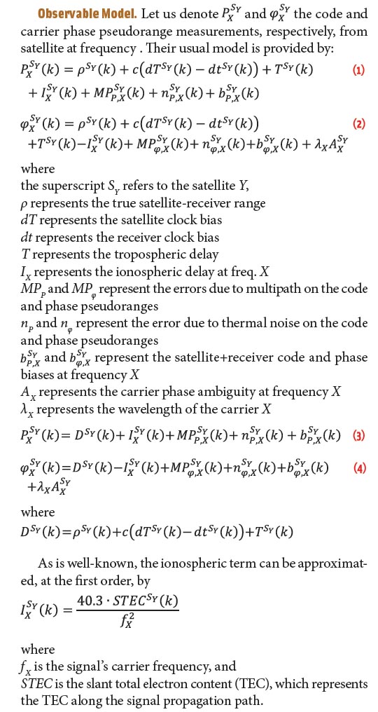
Observable Model.
Equations (1-4) (see inset photo, above right)
Ionosphere Estimation Techniques
The reference ionosphere delay estimation technique was fully presented in O. Julien et alia (2012); so, we will only briefly describe it here.
Dual Frequency Measurements. The ionosphere delay for each visible satellite can be estimated from two signals at two frequencies using dual-frequency code geometry-free combinations as follows:
In the case of an E5a and E5b combination, the coefficient KE5b, E5a equals 19.9 when estimating the ionospheric delay at E5a. This means that all the tracking errors (e.g., due to multipath, noise, interference) and hardware biases are multiplied by 19.9 when estimating the ionospheric delay. Clearly, this is very detrimental to the accuracy of the ionospheric delay estimation. So, let’s use dual frequency geometry-free carrier-phase combinations instead:
In this case, the multiplication factor is not as problematic because the carrier phase tracking errors are only at the millimeter/centimeter level. However, in this case, we must also estimate a float ambiguity term (coming from the carrier phase ambiguities):
Consequently, we must estimate the ambiguity terms together with the ionosphere term. As a result, the system has more unknowns than measurements.
Single-Frequency Measurements. If only one frequency is available, the ionospheric delay of each satellite can be estimated using the code-minus-carrier (CMC) combinations as follows:
Equation (7) takes into account the fact that code-tracking errors are two degrees of magnitude greater than the carrier phase tracking errors. As can be seen, the CMC combination also integrates the carrier phase ambiguities, and thus these ambiguities have to be jointly estimated with the ionosphere delay.
Local Ionospheric Model. To reduce the number of unknowns in the dual-frequency and single-frequency systems shown just described, we can try to use a simple local ionospheric delay model. This creates another advantage, which is to link the ionospheric delay terms associated with each visible satellite with a set of parameters to estimate.
Modeling the local variations of the vertical ionospheric delay around the user to facilitate the estimation of the ionospheric slant delay has been used for single-frequency (GPS L1 C/A) ionospheric estimation, as described in the articles by L. Lestarquit et alia and R. Moreno et alia). This method has also been used for dual frequency GPS L1/L2 measurements, as described by A. Komjathy in the context of precise point positioning (PPP) using a network of reference stations.
These methods assume that the ionospheric delays can be modeled using:
- a single layer ionospheric model such that each point of the ionosphere layer equals the VTEC
- a local VTEC model such that the VTEC at any ionospheric pierce point (intersection between the assumed single-layer ionosphere and the signal propagation path) can be modeled as a function of the VTEC at a specific reference point, and a VTEC gradient according to the difference in latitude and longitude between the pierce point location and the reference position
- a mapping function that maps the VTEC at the ionosphere pierce point into the STEC. A typical mapping function to transform the VTEC into an STEC is described in the article by L. Lestarquit et alia):
where
Re is the Earth radius (6378.1363 km)
E is the satellite elevation (in rad), and
hI is the height of the maximum TEC, which is also the height of the ionosphere layer modeled as a single-layer.
The authors tested nine simple local VTEC models derived from the foregoing general model and applied them to the case of a Galileo E5a/E5b receiver as described in the article by O. Julien et alia (2012). The selected model was based on the expression of the VTEC at the ionosphere pierce point as a function of the following parameters:
- the VTEC at the zenith of the user VTECu
- Four VTEC gradients in north gN, east gE, south gS, and west gW directions
- the considered latitude of the ionosphere pierce point and the user location is the geomagnetic latitude.
This local VTEC model can be represented as:
where
latu and latp are the user and pierce point latitudes, and
longu and longp are the user and pierce point longitudes.
Using the fact that the ionospheric delay at frequency X1 for satellite SY can be modeled as
Ionosphere Estimation Using Galileo E5 Only. The ionospheric delay estimation described by the authors in 2012 is based on a Kalman filter that uses (1) the dual-frequency code and carrier phase measurements as measurements, and (2) the local VTEC model parameters and the ambiguity terms as state parameters. The state matrix is thus:
Note that this system has the advantage of separating the inter-frequency phase bias from the ionospheric delay terms since the inter-frequency phase bias will be absorbed by the (float) ambiguity state once the filter has converged. The inter-frequency code bias might create a problem, although the estimation process will mostly be based on the carrier phase measurements.
The transition matrix is based on the following assumptions:
- The ionosphere-related terms are modeled as first-order Gauss-Markov processes.
- The ambiguity terms are modeled as first-order Gauss-Markov processes since these states will absorb the potential variation of the hardware biases as well as the ionosphere modeling error.
- The Earth rotation is taken into account to update the vertical ionospheric delay between two consecutive time updates.
The transition matrix associated with the reference local ionosphere model is thus
where
σVTEC, σGN, σGS, σGE, σGW, are the standard deviations associated with the variation of the local ionosphere parameters
σA corresponds to the standard deviation associated with the variation of the ambiguity term (mostly due to the ionosphere modeling error variation)
nVTEC, nGN, nGS, nGEE, nGW, nAs1, … , nAsn are independent Gaussian noise with a unit variance, and
WE is the Earth rotation rate (rad/s).
Ionosphere Estimation for Galileo E5/GPS L5. When using Galileo E5 and GPS L5, the estimation process must be amended since Galileo will provide dual-frequency measurements, while GPS will only provide measurements on L5. Using CMC measurements for GPS L5, the system to solve is now:
As it is easy to find the expression of the matrix H for this system from what was presented in the Galileo E5_only case, it will not be detailed here. The same deduction can be done regarding the transition matrix F.
Ionosphere Estimation for Dual Constellation/Dual Frequency. For references, a third test case was investigated. This test case aimed at assessing the performance of the estimation process in the case of Galileo E5 together with another constellation that would have two available signals in the E5 band. This case is interesting as it would allow using dual frequency carrier phase measurements instead of CMC measurements, which are much noisier. As a consequence, a ‘fictitious’ GPS constellation was used that assumed that GPS satellites were able to transmit an ALTBOC(15,10) on the same frequency as Galileo E5. By doing so, the idea was to test the estimation process using dual constellation dual frequency carrier phase measurements.
As in the case of Galileo E5/GPS L5, the Kalman filter equations can be deduced from what was presented in the Galileo E5 only case as the local VTEC model is assumed to be the same.
Local VTEC Model based on Three Gradients. In the authors’ work in 2012, the true VTEC variations obtained from the NeQuick model were analyzed. It was observed that there could be some potentially strong variations of the gradients in the North/South directions over Europe. This is why it was originally decided to have separate North and South gradients. However, the variation in the East/West direction appeared more linear. As a consequence, in the frame of this paper, another local VTEC model will be tested based on only three gradients: North, South, and East/West. The motivation for testing this model is to see how a model with fewer parameters will behave, in particular taking advantage of greater observability for each parameter.
The Simulation Tool and Filter Settings
The simulation tool is exactly the same as the one used by the authors in 2012. There are, however, several differences:
- The true ionosphere is now modeled using the NeQuick2 model, an evolution of the NeQuick model freely available on the ITU website and used in by ITU-Radionavigation’s “Reference Ionosphere Characteristics, Recommendation P.1239,” and in the articles by S. M. Radicella and M. L. Zhang, and R. Leitinger et alia listed in Additional Resources. For visualization purposes, the C/N0 for the considered Galileo E5 signal’s component at the user antenna output is shown in Figure 1. The difference between NeQuick1 and NeQuick2 is mainly that the variation of the VTEC is not as sharp in NeQuick2 as it is in NeQuick1 due to modifications in the modeling of the high-altitude ionosphere layers.
- GPS satellites are assumed to follow the GPS constellation defined in RTCA SC-159 document, “Assessment of Radio Frequency Interference Relevant to the GNSS L5/E5a Frequency Band.” The link budget associated with the GPS satellites takes into account the power output difference between GPS and Galileo signals.
- Multipath is generated assuming a single reflector (the Earth surface), and the user antenna located on a pole two meters above the ground.
Kalman Filter Settings. The observation noise variance was chosen to be the product of a C/N0-dependent term and an elevation-dependent term. The C/N0-dependent term is the usual theoretical tracking noise variance. The elevation-dependent variance represents the impact of multipath and was chosen to be equal to
The chosen covariance matrix for the process noise was set empirically to allow for a variation of 0.1 centimeter per second for the vertical ionosphere component, 0.5 centimeter per radian per second for the gradients, and 0.01 centimeter per second for the ambiguity terms.
Simulation Parameters. We chose a receiver mask angle of 10 degrees and selected five locations to represent a diversity of latitudes and longitudes:
- Sevilla, which is supposed to be close to the VTEC peak and should thus have higher VTEC gradients
- Toulouse, which is in the middle of Europe (in terms of latitude) and should have average VTEC gradients, and
- Stockholm, which is in the upper part of Europe (in terms of latitude) and should have low VTEC gradients
- Beijing, which sees an ionosphere activity that should be similar to Sevilla (see Figure 2)
- Shanghai, which is very close to the VTEC peak and can be considered as a worst-case scenario (see Figure 2).
We selected four time periods representative of the TEC during a plurality of ionosphere activities, which were drawn from the table of the monthly R12 indexes over the period 1931–2001 provided by ITU, as follows:
- May 1958, with an R12 value representing an extremely active ionosphere (99 percent of all the R12 values in the ITU table are lower.)
- May 1980, with an R12 value representing a very active ionosphere (95 percent of all the R12 values in the ITU table are lower.)
- September 2002, with an R12 value representing an active ionosphere (66 percent of all the R12 values in the ITU table are lower.)
- July 1998, with an R12 value representing a median ionosphere activity (50 percent of all the R12 values in the ITU table are lower.).
Simulation Results
We ran simulations for the five locations, in four time slots, and for all configurations (Galileo E5 only, Galileo E5/GPS L5, and Galileo E5/“fictitious GPS dual-frequency” — the latter configuration to make up for the fact that GPS does not use two frequencies in L5). Four results of the simulations are analyzed:
- the maximum ionosphere estimation error at L1
- the 68th percentile of the ionosphere estimation error at L1
- the 95th percentile of the ionosphere estimation error at L1
- the 99th percentile of the ionosphere estimation error at L1.
The ionosphere estimation errors are given at L1 as this is currently the typical reference frequency. In the following, the statistics are computed considering only the ionosphere estimation error of:
- all Galileo satellites above the receiver mask (10 degrees) and
- all Galileo satellites above 30 degrees, but with all satellites above 10 degrees used in the estimation system.
Table 1 presents the simulation results for the European cities for satellites above 10 degrees and Table 2, for satellites above 30 degrees, with the latter table showing only the results for the four-gradient local VTEC model. In these tables, the lowest values for a given day and location are in boldface type.
It generally appears that the best results are obtained when using two constellations with dual-frequency signal processing. The main advantage of this configuration over the Galileo E5 only configuration is to limit the occurrence of large errors as can be seen in the rows showing the maximum and 99th percentile of the ionosphere estimation errors. This is true mostly in the difficult cases (very high ionosphere activity).
This means that the use of the dual-constellation/dual-frequency case allows for a better assessment of the rising and setting satellites’ ionosphere delay, probably due to the fact that twice as many satellites are used and that the ionosphere sounding is thus more distributed around the user. However, for a quieter ionosphere, the results between the dual-constellation/dual-frequency and single-constellation/dual-frequency cases are quite comparable. The primary reason is that the main source of error of the proposed ionosphere estimation process in a quieter situation is the chosen model itself: the local VTEC model itself plus the mapping function.
The dual-constellation/dual-frequency configuration provides a worst-case ionosphere estimation error below two meters and a standard deviation of the ionosphere estimation error below 30 centimeters in the three European cities. When looking only at satellites above 30 degrees (see Table 2), these worst-case results show a maximum error below one meter and a standard deviation of the estimation error below 20 centimeters in the same three cities. This is an excellent result considering that these results include the top one percent of the strongest ionosphere activity.
Finally, the Galileo E5/GPS L5 configuration appears to provide the worst results. This is even quite significant for simulations in Toulouse and Sevilla where the ionosphere is more active. The main reason is that the GPS L5 CMC measurements are much more affected by multipath than Galileo E5a/E5b dual frequency carrier-phase measurements. This can create local errors that leak into the ionospheric parameters resulting in large estimation errors, particularly for low-elevation satellites.
From Table 1 it can also be seen that the choice of three or four gradients does not make much of a difference in the estimation process., thus validating that the VTEC is almost linear in the East/West direction.
Detailed Analysis of Results for Toulouse in May 1980. In order to understand the estimation process, a specific analysis of a test case is interesting. The test case chosen here is the case of Toulouse in May 1980. Figure 3 shows the number of visible Galileo and GPS satellites over the course of a day.
For the dual-constellation/dual-frequency configuration, Figure 4 and Figure 5 show the output of the estimation process (vertical ionosphere and gradients, respectively). The observation of the estimated gradient shows that while the estimated north and south gradients can differ quite significantly, thus justifying the use of two different parameters, this is not the case for the east and west gradients that tend to remain within the same value. This explains why the cases of three and four gradients in the estimation process do not lead to significantly different results.
Figure 6 represents the actual ionosphere estimation error at L1 for the Galileo satellites. It can be seen that the major errors are coming from rising and setting satellites, while when the satellites are at medium to high elevation, the estimation error is almost systematically below 0.5 meter.
Figure 7 and Figure 8 show the ionosphere delay error as a function, respectively, of the ionosphere pierce point longitude and geomagnetic latitude with respect to the user location. Here we can see that the highest uncertainty seems to come in the latitude (north/south) since the plots are distributed over a wider area. On the other hand, in the east/west direction (longitude), a trend seems to show up as a second-order function in which the ionosphere error appears to grow as the difference between the longitude of the pierce point and of the user increases. This may mean that a more optimal local VTEC could be found.
Other local VTECs were tested to take into account this observation, in particular by adding a second-order coefficient for the gradients. However, no improvement was noticeable in other tested configurations. We believe that the use of a more optimal local VTEC model might only bring marginal improvement because an uncertainty also exists regarding the actual accuracy of the STEC mapping function when the ionosphere is very active.
Analysis of Results in Asia
Table 3 and Table 4 show the results for Beijing and Shanghai only for the dual-frequency cases and only for the four-gradient local VTEC model. The tables indicate that the results in Beijing are similar to those in Europe, which is not surprising as the locations have a similar geomagnetic latitude.
However, Shanghai shows very large estimation errors with worst-case situations reaching almost five meters (more than 60 centimeters standard deviation). This is due to the difficulty for the proposed linear VTEC model to accommodate the vicinity of the VTEC peak, creates large non-linear variations. Still, the results can be seen as reasonable given the conditions.
Conclusions
This article has shown further results to the ionosphere delay estimation process that was presented in 2009 and 2012 by the current authors as well as in the article by Sahmoudi et alia. In particular, this article is based on a more representative ionosphere condition due to the use of the latest NeQuick model for the simulations. It also proposed the use of a new local VTEC model and new receiver configurations.
The simulation results demonstrate that the proposed ionosphere estimation process, when having access only to the E5 band and to two constellations with two frequencies in the band, can produce quite interesting results for European locations even in the case of a very active ionosphere. Indeed, the data indicate that in one of the worst-case situations (top one percent of the greatest ionosphere activity), the standard deviation of the ionosphere estimation error at L1 was less than 30 centimeters for satellites above 10 degrees elevation and below 20 centimeters for satellites above 30 degrees. The results also showed that the maximum error was around two meters (and below one meter 99 percent of the time).
The results proved very interesting even if only one dual-frequency constellation (Galileo) was available in the E5 band. A substantial performance degradation with respect to the dual-constellation configuration was only seen for extremely active ionosphere conditions.
However, the use of a second constellation with only one signal in the E5 band did not appear to be very beneficial, as it increased the estimation error due to the use of CMC measurements. The limitation of the model was also highlighted when the user location becomes too close to the VTEC peak location because in those cases the simple linear local model cannot accommodate large and steep VTEC variations in several directions.
Additional Resources
[1] Bastide, F., “Analysis of the Feasibility and Interests of Galileo E5a/E5b and GPS L5 Signals for Use with Civil Aviation,” Ph.D. thesis, 2004
[2] European Union, European GNSS (Galileo) Open Service Signal-in-Space Interface Control Document
[3] ITU-R, “Reference ionosphere characteristics, Recommendation P.1239” (approved in 1997/05, managed by ITU-R Study Group SG3)
[4] Julien, O., and Macabiau, C., Issler, J-L., and L. Lestarquit, “Ionospheric Delay Estimation Strategies Using Galileo E5 Signals Only,” Proceedings of the ION GNSS 2009, Savannah, Georgia, 2009
[5] Julien, O., and Issler, J-L., and L. Lestarquit, “Ionospheric Delay Estimation Using Galileo E5 Signals Only,” Proceedings of the ION GNSS 2012, Nashville, Tennessee, 2012
[6] Komjathy, A., “Global Ionospheric Total Electron Content Mapping using the Global Positioning System,” Departments of Geodesy and Geomatics Engineering, University of New Brunswick, Fredericton, New Brunswick, Canada, Ph.D. thesis, 1997
[7] Leitinger, R., and M. L. Zhang, and S. M. Radicella, “An Improved Bottomside for the Ionospheric Electron Density Model NeQuick,” Annals of Geophysics, Vol. 48, No. 3, pp. 525–534, 2005
[8] Lestarquit, L., and G. Artaud, and J-L Issler, “ALTBOC for Dummies or Everything you Always wanted to Know about ALTBOC,” Proceedings of the ION GNSS 2008
[9] Lestarquit, L., and N. Suard, and J.-L. Issler, “Determination of the Ionospheric Error using only L1 Frequency GPS Receiver,” Proceedings of the 1997 ION National Technical Meeting, Santa Monica, California, January 14-16, pp. 313-322, 1997
[10] Moreno, R. and N. Suard, “Ionospheric Delay Using Only L1: Validation and Application to GPS Receiver Calibration and to Inter-Frequency Biases Estimation,” Proceedings of the 1999 ION National Technical Meeting, San Diego, California, January 25-27, pp. 119-125, 1999
[11] Radicella, S. M. and M. L. Zhang, “The Improved DGR Analytical Model of Electron Density Height Profile and Total Electron Content in the Ionosphere,” Annals of Geophysics, Vol 38, No. 1, 1995
[12] RTCA SC-159, Assessment of Radio Frequency Interference Relevant to the GNSS L5/E5a Frequency Band, RTCA DO 292, July 2004
[13] Sahmoudi et alia, “U-SBAS: A Universal Multi-SBAS Standard to Ensure Compatibility, Interoperability and Interchangeability,” NAVITEC Conference, Noordwijck, December 2010
[14] Simski, A., J.-M. Sleewaegen, M. Hollreiser, and M. Crisci, “Performance Assessment of Galileo Ranging Signals Transmitted by GSTB-V2 Satellites,” Proceedings of the 2006 Institute of Navigation GPS Conference, Albuquerque, NM, September 16-18,, pp. 483-490, 2006
[15] Van Dierendonck, A. J., “GPS Receivers” in Global Positioning System: Theory and Practice, B. Parkinson and J. J. Spilker Jr., Eds., Washington DC, AIAA, 1996