
Detecting interference using machine learning algorithms to monitor ADS-B data.
Zixi Liu, Sherman Lo, Todd Walter, Stanford University
GNSS serves several safety-of-life applications in aviation. It is used to support precise navigation for approach and landing operations. Additionally, it supports surveillance, Air Traffic Control (ATC) and collision avoidance by providing awareness of the traffic situation, allowing for safe management of aircraft interaction. Therefore, the loss of GNSS could severely affect the safe operations of the airspace, particularly for aircraft losing GNSS signals on approach or landing. A system that can quickly detect GNSS interference and provide ATC situational awareness can protect the safe use of GNSS in aviation. One way to detect the existence of a jamming event is by monitoring the Automatic Dependent Surveillance—Broadcast (ADS-B) reports from the aircraft.
ADS-B is a surveillance system onboard the aircraft that broadcasts the GNSS derived position at regular intervals. Messages may be transmitted using several protocols, with Mode-S Extended Squitter (Mode S ES) on the 1090 MHz frequency band the primary means worldwide. The broadcasted messages can be received by any ADS-B receiver in the area, such as those installed on many aircraft and ground stations. Nearly all aircraft in Europe and the U.S. were required to add the receivers by 2020, so ADS-B is already used by commercial aircraft extensively. The ubiquity and openness of ADS-B provides a widely available source of GNSS information from aircraft.
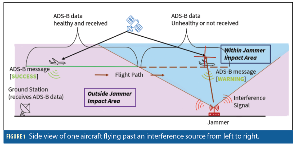
RTCA DO-260B [1] specifies the standards for ADS-B avionics. It indicates that if GNSS is unavailable but barometric altitude is, ADS-B should continue transmission and send a Type 0 position report. Furthermore, according to RTCA DO-181D (EUROCAE ED-73C) [1], the standards for air traffic transponder signals, if no new GNSS position data is received within 2 seconds of the previous data update, the ADS-B transmitting subsystem will clear all position information on the aircraft, except for the altitude and status subfields of the airborne position message. While the position information for the ADS-B message transmission may be based on other navigation systems, currently only GNSS has been accepted as an adequate source to provide relevant accuracy and integrity data for ADS-B. Hence, when non-GNSS sources are used, the quality indicators describing the integrity and accuracy of position data should indicate the lack of these measures. Therefore, we can expect to observe a loss of airborne position and/or a decrement of accuracy and integrity as the aircraft enters the area impacted by interference. Figure 1 shows how an interference event may affect aircraft GNSS reception and hence ADS-B outputs.
There are several types of ADS-B messages that come at different rates: position, velocity and operational status. Airborne position and velocity messages are typically broadcast every 0.4 to 0.6 seconds while the operational status message is sent every 2.4 to 2.6 seconds. These messages do not contain explicit receiver information, such as carrier to noise ratio (C/N0), however, they have built-in parameters that indicate the accuracy and integrity level of the reported information.
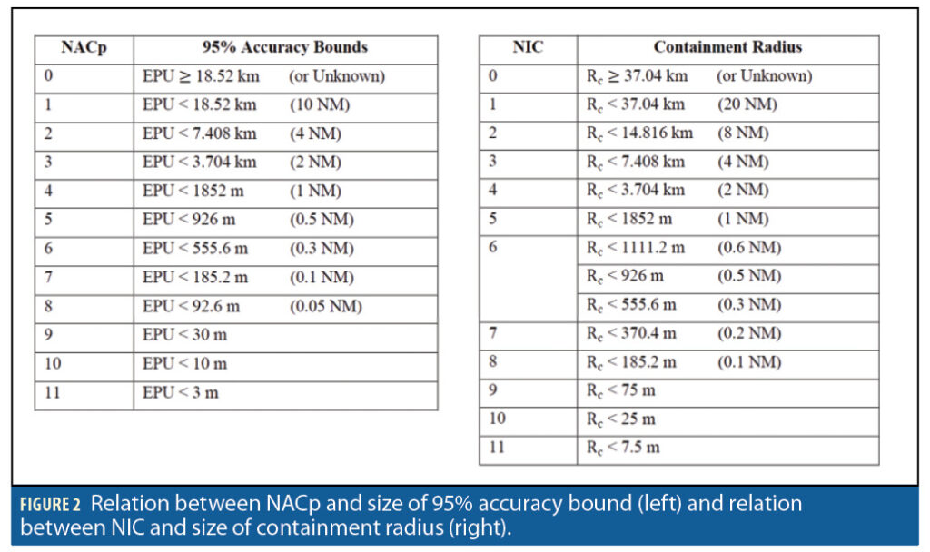
Two commonly used parameters are Navigation Accuracy Category–Position (NACp) and Navigation Integrity Category (NIC). NACp is sent with an ADS-B operational status message. It provides an estimate of the horizontal and vertical position uncertainty (EPU) of the provided ADS-B position solution. The physical meaning behind the parameter is the size of 95% accuracy bound on the current reported position. Imagine drawing a sphere centered at the reported position; the actual position should be somewhere within the sphere, with probability greater than 95% under all nominal conditions. Therefore, a larger sphere radius means a larger bound on worst-case errors and worse information quality.
NIC is sent with an ADS-B position message. NIC specifies an integrity containment radius that the current position is guaranteed to be within the horizonal protection level of a specified containment radius with 99.999% probability. Figure 2 shows the tables for NACp and NIC. On the left is a table for NACp and its corresponding 95% accuracy bound. On the right is a table for NIC and its corresponding size of containment radius [1]. The corresponding error or containment value for low values NACp or NIC (i.e. 0) are much worse than typical GNSS performance. For example, for a NACp or NIC value of 0, the accuracy and integrity level provided essentially indicates they are unknown. For GNSS to perform this poorly, the aircraft likely has been severely affected by the jammer.
The main purpose of this project was to design a system that could rapidly identify and narrow down possible areas of interference events. We were inspired by the idea of using convolutional neural networks (CNN) to perform object detection in image processing. We designed and trained a CNN model to detect impacted regions within an airspace in a manner analogous to detecting an object from an image. Figure 3 is an overview of the designed system.
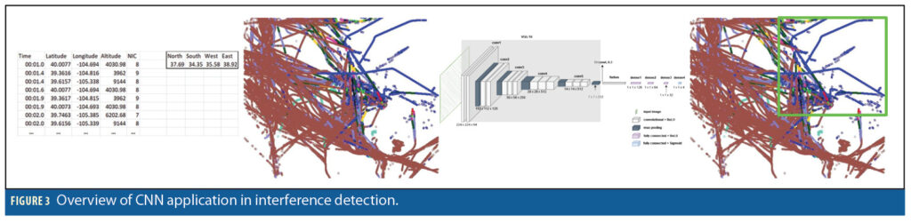
Given a selected airspace, which may or may not contain an interference event, we first collected ADS-B position messages from all aircraft flying through that airspace. We then plotted the overall picture of all the flight paths from the collected ADS-B data. The CNN model took this overall picture as an input and output the corresponding bounding box that indicates the affected region. This bounding box contains information about the latitude and longitude coordinates of the north, south, west and east boundary.
Using CNN to detect the existence of interference events as well as identify the bounding box of the affected region is a starting point for improved detection and localization, especially when the size of the suspected airspace is large. For instance, if we are looking for interference events happening around the entire world, it may be cumbersome to manually identify them all. However, we could input the overall picture of all aircraft flight paths into the CNN model and immediately get results showing which regions contain interference events.
In addition, current solutions for interference detection and localization (IDL), such as radio direction finding, are generally costly and time-consuming when the search area is large. Therefore, narrowing down the possible areas of interference events can help speed up the process. It also can help speed up some more refined localization algorithms that may get stuck at a local minimum when initiated too far away from the true jammer location. Furthermore, the CNN model can process information that might be difficult to represent using simple and low computation mathematical models. For instance, missing part of a flight path is one possible outcome from an interference event, but if there’s a mountain between the aircraft and the ground ADS-B receiver, that could also cause gaps on the flight track. It may be difficult to mathematically distinguish between these two scenarios, but the CNN model can be trained to do so.
Related Work
Some researchers have done similar work on detection and localization of GNSS interference events using ADS-B data. Most of the prior works focus on solving problems from the signal transmission perspective as well as statistical analysis. There are only a few works that cover using ADS-B data to perform interference detection and localization because of the coarseness and challenges with the data. Therefore, we applied machine learning algorithms to address this problem rather than rely on simple, low computation mathematical models.
As for interference detection, Aireon provides alerts of potential GPS interference events by monitoring a change of NACp from the ADS-B messages [2]. In this effort, we used NIC as an input parameter. This decision was made based on some of our previous studies in characterizing ADS-B performance during interference events [3]. NIC comes with the position message directly, while NACp is part of the operational status message that is broadcast less frequently. Therefore, using the NIC value ensures each position point will have an associated quality indicator.
As for localization, EUROCONTROL has investigated the use of ADS-B to localize GNSS interference based on the position information outages within flight paths. They developed a grid probability model to calculate and generate heatmaps for possible location of the RFI source [4]. As a starting point, we proposed using convex optimization to identify possible location of the interference source [5]. The main idea is to minimize the distance between the outer boundary of the jammer impacted region and the starting position of flight path outages. This is based on the assumption the aircraft loses GNSS reception immediately after entering the jammer impacted region. Other assumptions were made, such as the interference source was omnidirectional, and there was no ADS-B signal blockage from mountains or buildings, meaning gaps within the flight tracks were only from jamming. These assumptions led to a mathematical model that is overly idealistic when applied in real-life events. This project addressed those deficiencies by designing a CNN model trained on data collected from real-life interference events, making it more applicable.
The Dataset
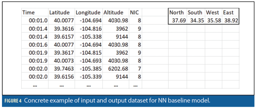
This project uses ADS-B data queried from OpenSky Network, a community-based receiver network [6]. For our baseline model, we used structured data shown in Figure 4. Each row contains aircraft position information at one time stamp, and each column corresponds to one feature. We chose five features for this project: latitude, longitude, altitude, time and NIC. The dataset output label is a bounding box of the impact region represented by the latitude or longitude value of the edges.
Real Data
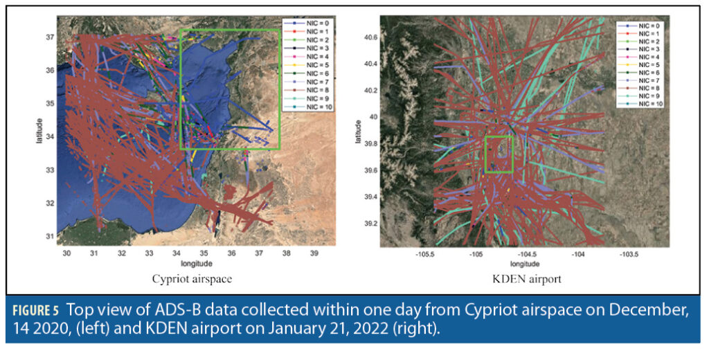
We used images as input data for our CNN model by plotting aircraft flight paths onto Google Maps. We ran our algorithms on two different sets of data. The first set of data is ADS-B reports collected from real-life interference events. We queried ADS-B data from interference events that occurred in the Cypriot airspace from December 13, 2020, to December 20, 2020. There is ongoing significant and known GNSS interference that occurs in that airspace [7]. The possible location of the interference source was identified by C4ADS using satellite data [8]. This report aids our analysis by providing an educated guess on the location of the interference signal. In addition, we also collected ADS-B data from another interference event that happened at the Denver International Airport (KDEN) from January 20, 2022, to January 23, 2022. The interference source was identified by the U.S. Department of Transportation, which provided information about the jammer location and power.
Figure 5 shows a top view of all flight paths observed in one day from Cypriot airspace (on the left) and Denver airport (on the right). All the dots are position messages received from aircraft that include latitude, longitude and altitude. The color of each dot represents the corresponding NIC value. For instance, position message with NIC = 0 is blue. The green bounding box is the truth label of the impact region. The location and size of the bounding box is determined based on interference source information. The center of the box is the jammer location and the size of the box indicates the jamming power.
Simulated Data
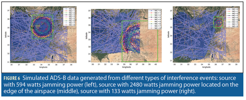
The CNN model requires training on manyimages. However, we only had a few days of overall pictures from real-life events. And within each airspace, there is only one static interference source with one constant location among different days. That means no matter how many days of datasets we collected, there is only one underlying class label that corresponds to that one static location of the interference source. Therefore, we used simulated data for additional training. The simulator can produce different overall pictures caused by different jammer locations and different jamming powers. Figure 6 shows a few sampled plots of the simulated data.
The main purpose of this simulator is to help create different types of interference events such as jammers with different power levels, as it is difficult to find real-world ADS-B data that has a known jammer location and an adequate density of points in all directions about the jammer. In addition, we want our CNN model to learn properties we observed during real-life events; therefore, we simulated multiple overall pictures of those cases to sufficiently train the model. For instance, we noticed incorrect operation of the on-board ADS-B system could lead to the NIC value always equaling zero. We also noticed some noise within the NIC value as some flight values jumped between 6 and 7 under nominal conditions. Therefore, during simulation, we randomly added flights with NIC values always equal to zero, as well as some noise to the flights with an NIC of 7s. We generated 5,000 days of ADS-B data from different types of interference events.
Baseline
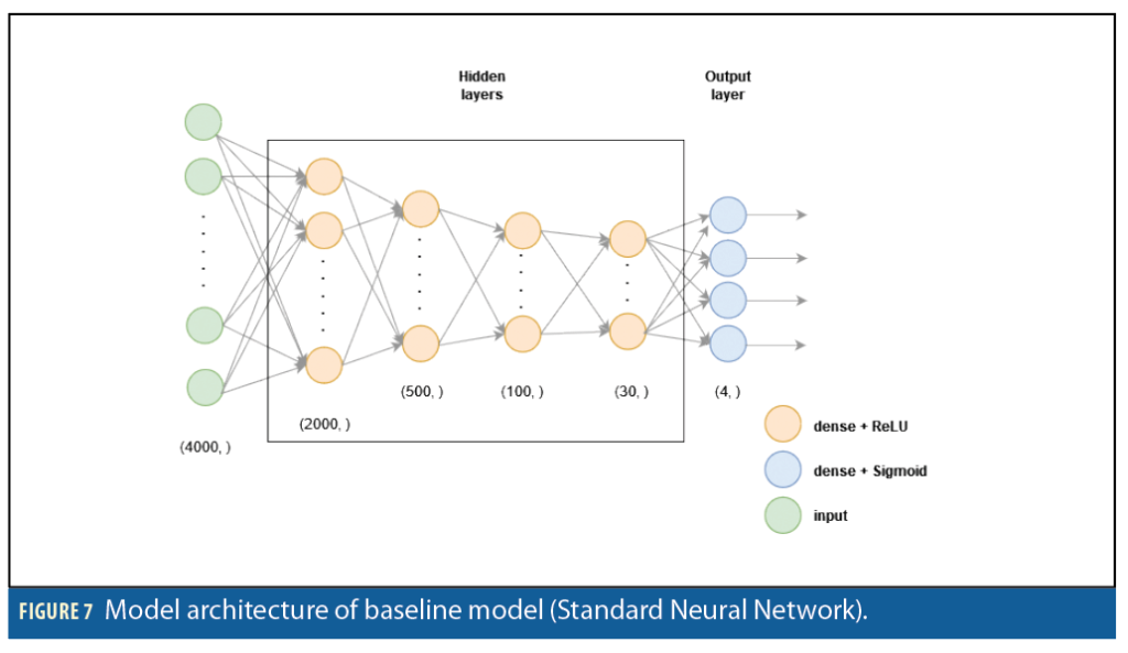
In this effort, we used standard neural network as our baseline model. Figure 7 shows the designed structure of our baseline model. Each training example contains information from 1,000 position messages each including latitude, longitude, altitude and NIC. Therefore, it has been reshaped into a vector of size (4000,). The output value is a vector of size (4,), which has latitude and longitude information of the affected region, or the north, south, west and east side of the bounding box. We trained this model using stochastic gradient descent with a learning rate of 0.001 and a batch size of 32 for 20 epochs.
Main Approach
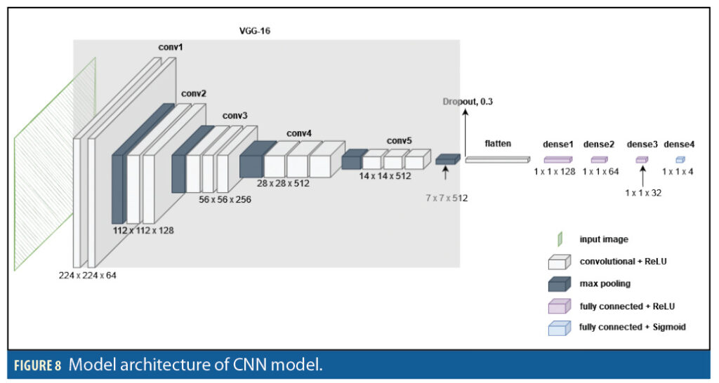
We were inspired by the idea of using CNN to perform object detection. This project applied transfer learning using a pre-trained VGG16 model [9], which is a common and powerful CNN architecture developed for computer vision. In addition, we used Keras [10] to build our machine learning model, which is a powerful and easy to use Python library. Figure 8 shows the architecture of our CNN model. The input is an image of size (224, 224, 3) that contains all flight paths within one day. The output value is a vector of size (4,) which shows the boundary location of the impact region in the format of latitude of south edge, latitude of north edge, longitude of west edge and longitude of east edge. We trained this model using the Adam optimization method [11], which accelerates the convergence toward the relevant direction and prevents the vanishing gradient problem, with a learning rate of 0.0001 and a batch size of 64 for 20 epochs.
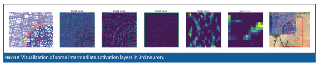
To better understand the performance of the CNN model, we also created a visualization of intermediate activation layers. This helped us understand what features were extracted from the image by each layer and each unit. Figure 9 shows how the input image has been learned and how the interference region has been identified by the model. We can see the starting layers correspond to low-level features like flight paths, whereas the later layers look at high-level features such as the regions with low NIC values that are closer to the jammer.
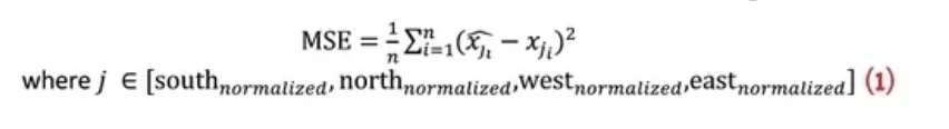
Quantitatively, we evaluate models using mean squared error (MSE). Because we generated outputs of latitude and longitude that are continuous numbers, it is proper to evaluate regression models using the average of the squares of the errors. MSE is an absolute measure of the goodness of the fit; the smaller it is, the better the model fits the training data.
Qualitatively, we evaluated models using R-squared. R-squared is a relative measure of how well the model fits dependent variables; the higher the R-squared value is, the better the model explains the variance of data. An R-squared value of 1 means the model fits the data perfectly. Notice we want to avoid negative R-squared value, which means the fit is worse than just fitting a horizontal line to the data.
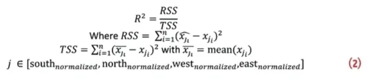
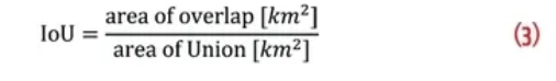
The true label and the predicted label are normalized into values between 0 and 1. Therefore, the MSE and R-squared values are unitless and used as relative measurements of how to tune the hyperparameters of the model. To have an intuitive understanding of how well the predicted bounding box matches with the truth label, or in other words, to understand the physical meanings behind the predicted result, we calculated the area formed by the predicted and true bounding box. We then calculated the intersection over union (IoU), which is the ratio of area overlapped by the two bounding boxes to the union area formed by the bounding boxes. IoU evaluates the degree of overlap between the predicted and truth bounding box. It ranges from 0 to 1 and 0 means no overlap.
Experiments
We performed a set of experiments on some of the important hyperparameters of the models, including learning rate, optimization methods, dropout rates, and sample weights. We ran k-fold cross validations on 500 images that were trained with 80% of data and validated on the remaining 20%.
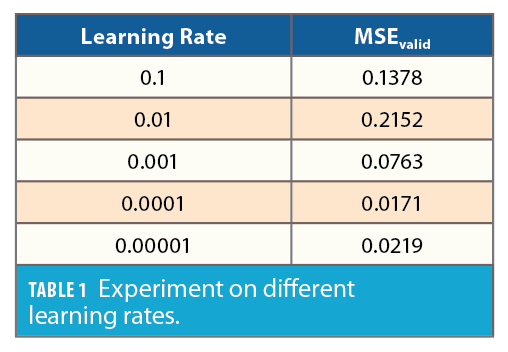
For all experiments, it’s important to find properties that have a high tendency to reduce validation MSE. Our model tends to converge too quickly to a sub-optimal solution if we use a large step size. Table 1 illustrates how learning rate affects validation MSE. Notice learning rate 0.1 has better results than 0.01. However, if we keep decreasing the learning rate, the 0.1 result is just a local sub-optimal solution. Our final choice is to use a learning rate of 0.0001.
We noticed the potential risk of trapping at local minima, but using a small learning rate might lead to slow convergences. Therefore, we ran experiments on different optimization methods and found the Adam optimization method not only has the smallest MSE, but also the highest tendency to decrease the error as the number of epochs increases. This is expected because the Adam optimization method accelerates convergence toward the relevant direction and prevents the vanishing gradient problem.
In addition to reducing the model bias, we also wanted to reduce the variance as we noticed the validation error is always higher than the training error. Therefore, we added a dropout layer. We found a dropout rate of 0.3 helps reduce the validation error most and therefore became our final choice for the dropout layer.
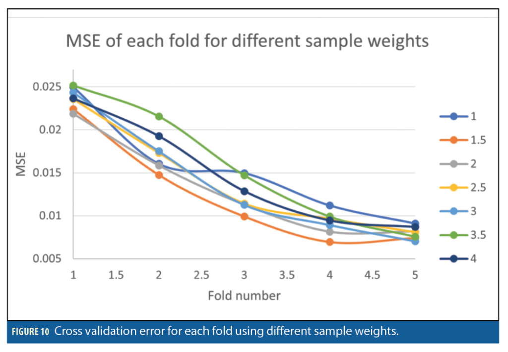
Lastly, because our model is trained using both simulated and real datasets, it is important to solve the domain adaptation problem by adding weights to the real data. We ran k-fold cross validation on the entire dataset with K = 5. Figure 10 indicates how adding more weights to the real-life data affects the error. Notice that for the 3rd, 4th, and 5th fold of validation set, adding sample weights is always better than no sample weights, as they all reduce the cross-validation error. However, for the 1st and 2nd fold of validation set, only sample weights of 1.5 and 2 can reduce the error. Because we want our model to work well on real-life data, larger sample weight is preferable. Therefore, we chose a sample weight of 3 as our final design.
Results and Analysis
The final mean squared error obtained from the test set for the baseline model and the CNN model are 0.0105 and 0.00305, respectively. Our CNN model improves the overall accuracy and better fits the bias of the data. The R2 value for the baseline model and CNN model are 0.3373 and 0.7977. Our CNN model has much higher R2 value than the baseline model and has reasonable fit to the variance of the data.
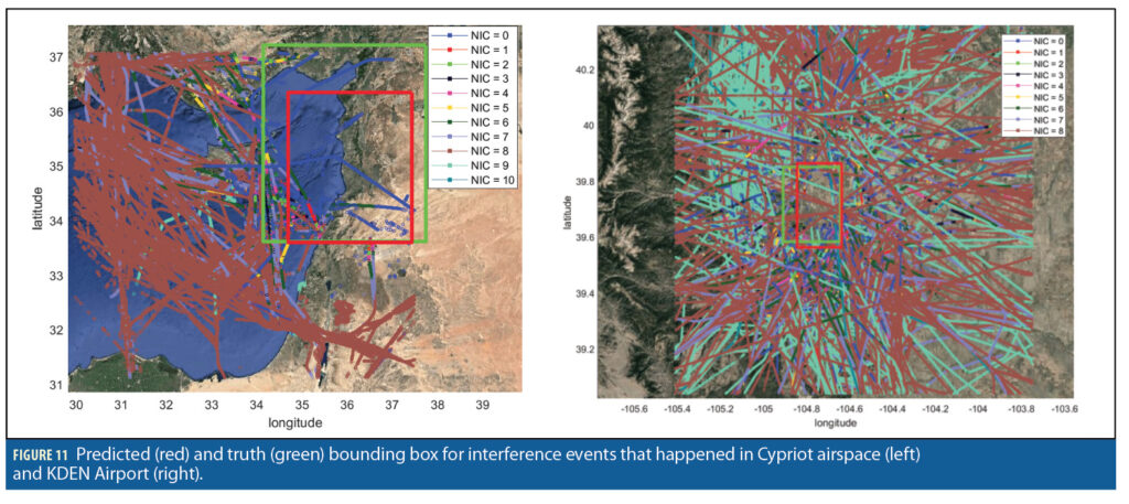
Figure 11 shows how our final model works on real-life data. The red box is a predicted bounding box and the green box is the true bounding box. On the left is the result for events in Cypriot airspace. The area of the predicted bounding box is around 76,000 km2 and the IoU is around 0.6. Because the predicted bounding box is contained by the true bounding box, an IoU of 0.6 means the size of the predicted bounding box is about 60% of the area of the true bounding box.
On the right is the result for the event at the KDEN airport. The area of the predicted bounding box is around 542 km2 and the IoU is around 0.8. Notice the predicted bounding box is always close to but smaller than the true bounding box. This is as expected because we don’t have much training data from real interference events. Therefore, the model could only roughly locate the interference source with slightly incorrect size.
When looking at the overall picture of flight paths from KDEN airport, (Figure 11, right), it seems the impact area should be as large as the entire airspace. However, the predicted and true bounding boxes are all quite small. This is because we plotted the impact area with respect to the ground location based on the known jammer power. Therefore, the true bounding box is smaller than what we would observe from the aircraft, which can be affected at much larger distances.
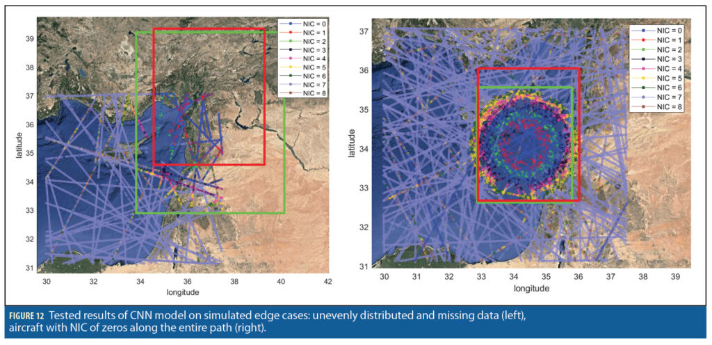
In addition to testing our model on real-life data, we also needed to analyze it through simulated edge cases in which the size of the interference region could be easily misidentified, even by humans. Figure 11, left, shows the result of testing on the first edge case, which is unevenly distributed data or missing data points. For our data, this is mainly from the lack of the ADS-B receiver ground coverage or mountains blocking the signals between aircraft and ground receivers. However, such missing data could be confused with loss of GNSS signals caused by the jammer. The area of the predicted bounding box is around 221,960 km2 and the IoU is about 0.54. The size of the predicted bounding box is smaller than the size of the true bounding box, but the relative location of the box is close to the correct location of the jammer impacted region. This means the model can identify the impact region but the missing information from the lack of ground coverage can cause a reduction in confidence or in the size of the output bounding box.
An NIC of zero along the entire path (Figure 12, right) is the second edge case. The incorrect operation of the on-board ADS-B system could lead to an NIC value that always equals zero. However, seeing multiple low NIC values causes confusion in an ADS-B based interference detection system as to whether the region has been affected by a jammer. The area of the predicted bounding box is around 107,860 km2 and the IoU is around 0.8. Notice the size of the predicted bounding box is slightly larger than the true bounding box, but the incorrect drop of NIC values does not drag the box toward these low NIC value areas. This means the model can identify false positives.
Conclusion and Future Work
In this project, we designed and trained a CNN model for interference event detection and localization. Given an airspace where interference events exist, by only collecting and feeding ADS-B data from the airspace into those trained models, we identified the size and location of the impact region. Using CNN to identify a bounding box around the affected region is a starting point for further improved detection and localization. It helps narrow down possible areas of interference events. This result can speed up the searching process, prevent algorithms from stopping at local minimums, and provide a reasonable initial point for implementing optimization methods.
In the future, we would like to further train our CNN model with more real-life data instead of simulated data. This requires obtaining datasets from interference events that contain jammer location information. This requirement is difficult to satisfy because not all GPS interference testing events provide information about the interference source. But if obtained, we expect our test result on real-life data would be as good as the result obtained in this project using both simulated and real-life data. Our current CNN model also can be easily transferred into a model that identifies the most likely location of the interference source.
Acknowledgments
The authors thank the FAA for sponsoring this research and OpenSky Network for providing ADS-B data.
This article is based on material presented in a technical paper at ION GNSS+ 2021, available at ion.org/publications/order-publications.cfm.
References
(1) DO-260B RTCA (Firm). (2011). “Minimum operational performance standards (MOPS) for 1090 MHz extended squitter automatic dependent surveillance – broadcast (ADS-B) and traffic information services-broadcast (TIS-B)”. Washington, DC: RTCA, Inc.
(2) Michael, G., “Global Surveillance and Tracking of Aircraft via Satellite”. presented to SCPNT Symposium, Stanford University, CA, USA, October 28, 2020. [PowerPoint slides].
(3) Liu, Z., Lo, S., and Walter, T., “Characterization of ADS-B Performance under GNSS Interference,“ Proceedings of the 33rd International Technical Meeting of the Satellite Division of The Institute of Navigation (ION GNSS+ 2020), September 2020, pp. 3581-3591.
(4) Jonáš, P. and Vitan, V., “Detection and Localization of GNSS Radio Interference using ADS-B Data,“ 2019 International Conference on Military Technologies (ICMT), Brno, Czech Republic, 2019, pp. 1-5.
(5) Liu, Z., Lo, S., and Walter, T., “GNSS Interference Characterization and Localization Using OpenSky ADS-B Data,” Proceedings 2020, 59, 10. https://doi.org/10.3390/proceedings2020059010
(6) Schäfer, M., Strohmeier, M., Lenders, V., Martinovic, I., and Wilhelm, M., “Bringing up OpenSky: A large-scale ADS-B sensor network for research,” In Proceedings of the 13th International Symposium on Information Processing in Sensor Networks, Berlin, Germany, April 2014.
(7) EUROCONTROL (2021, March 01). “Does Radio Frequency Interference to Satellite Navigation pose an increasing threat to Network efficiency, cost-effectiveness and ultimately safety?” Aviation Intelligence Unit, Think Paper #9. https://www.eurocontrol.int/sites/default/files/2021-03/eurocontrol-think-paper-9-radio-frequency-intereference-satellite-navigation.pdf
(8) Center for Advanced Defense Studies. Above Us Only Stars: Exposing GPS Spoofing in Russia and Syria. Washington, DC: C4ADS, 2019. https://www.c4reports.org/aboveusonlystars.
(9) U.S. Department of Transportation, Aviation Cyber Initiative PNT Meeting Briefing. February 10, 2022. [PowerPoint slides].
(10) K. Simonyan and A. Zisserman, Very Deep Convolutional Networks for Large-Scale Image Recognition. arXiv, 2014. doi: 10.48550/ARXIV.1409.1556.
(11) Chollet, F., others. (2015). Keras. GitHub. Retrieved from https://github.com/fchollet/keras.
(12) Kingma, D. P. and Ba, J., “Adam: A Method for Stochastic Optimization”, <i>arXiv e-prints</i>, 2014.
Authors
Zixi Liu is a Ph.D. candidate at the GPS Laboratory at Stanford University. She received her B.Sc. degree from Purdue University in 2018 and her M. Sc. degree from Stanford University in 2020.
Sherman Lo is a senior research engineer at the GPS laboratory at Stanford University.
Todd Walter is a professor of research and director of the GPS laboratory at Stanford University.