 Equations
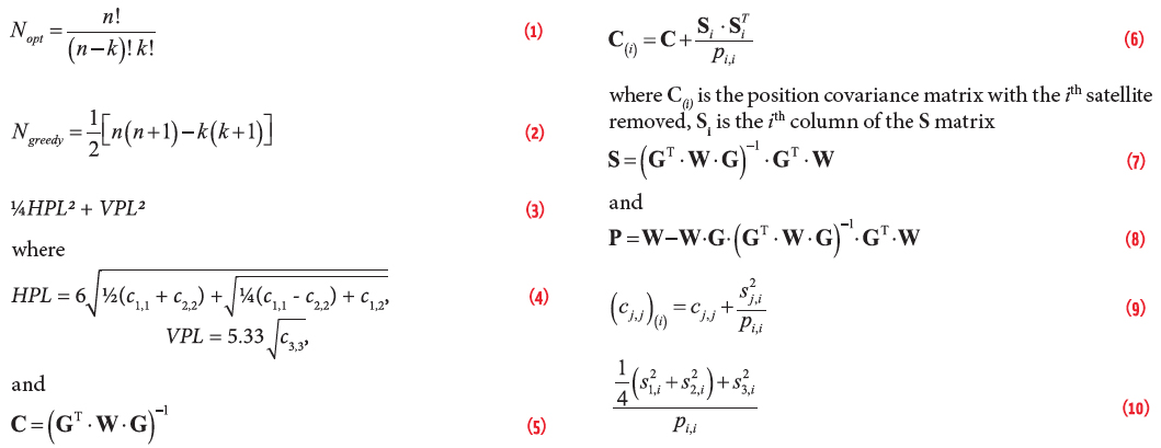 Equations
Working Papers explore the technical and scientific themes that underpin GNSS programs and applications. This regular column is coordinated by Prof. Dr.-Ing. Günter Hein, head of Europe’s Galileo Operations and Evolution.
Working Papers explore the technical and scientific themes that underpin GNSS programs and applications. This regular column is coordinated by Prof. Dr.-Ing. Günter Hein, head of Europe’s Galileo Operations and Evolution.
Radio frequency interference (RFI) is a serious threat not only for users of satellite-based services, but also for the satellite-based systems themselves. The impacts of RFI at the user level range from temporarily affecting the quality of service of non-critical user applications over a limited or wide area (e.g., the quality at which some users are watching a football game) to affecting the quality of service of safety critical applications (e.g., avionics applications). At the system level, RFI can cause degradation in the quality of the satellite based services (i.e., increasing the demodulation error of uplinked data with temporary loss of a satellite’s availability) or even causing long-term service degradation.
The emission types can be categorized as intentional (jamming or spoofing) and unintentional. Nowadays, most of the RFI affecting satellite communication services is not intentional. (For an examination of satellite interference sources including those on GNSS signals, see the presentation by R. S. Jakhu listed in Additional Resources near the end of this article.) Unintentional interference cases are expected to increase in coming years with the constant increase of satellites in orbit, the congestion of already crowded frequency bands due to the new deployment of terrestrial and space systems, and the current trend in reducing equipment and installation cost (mainly in commercial systems). Moreover, intentional interference is increasing dramatically due to the availability of low-cost jamming devices on the market.
Different strategies can be adopted to handle interference, as shown by Figure 1:
- monitoring: monitoring emission over an identified frequency range;
- detection: detecting the presence of interference that can degrade the system performance;
- characterization and classification: estimation of the main characteristics of the interfering signals, including the classification of the interfering signals within pre-defined classes of signals;
- mitigation: all steps to counteract the interfering signal, e.g., interference nulling;
- location measurements: extraction of location-dependent measurements from the interfering signals;
- localization: locating the interference sources via location algorithms that find these sources by processing the location measurements.
Localizing the source of RFI is becoming a priority in today’s satellite industry. Indeed, although much effort has been placed at the user level to design interference mitigation schemes to increase the system’s robustness in the presence of RFI on downlink signals, little has been done at the satellite level (i.e., on the uplink communication channel between a ground station and a satellite), whose local vulnerability propagates as a vulnerability in the entire system.
In this context, interference mitigation schemes can be useful to improve the performance of the system in the presence of RFI, but they cannot deter such type of threats from appearing in the future. Instead, interference localization provides the required essential information to the authorities on the location of the RFI source and time of such interference events, enabling them to stop the interference and prevent it from recurring.
This article continues a discussion begun in the Working Papers column in the November/December 2016 issue of Inside GNSS that addressed the theoretical background of interference localization. The current article focuses on the application of the techniques presented in that article to localize an interference source exploiting ground-based or space-based architectures.
Interference on Downlink Signals
The degradation of satellite downlink signals by means of interference directed to on-ground equipment is a well-known issue that must be taken into account in the receiver design. In this scenario, the interference signal arrives at the antenna elements of on-ground devices (e.g., user equipment) with a power and band such that it can affect the reception of downlink communications addressed to those devices. This type of interferer usually affects only a few devices in a limited area; nonetheless, this area could include critical infrastructure such as an airport.
Historically, intentional interferers are common for military scenarios. However, due to the availability of low-cost jamming devices on the market, intentional interference of civil applications is becoming common as well, although most remains unintentional. The latter interference stems from the large number of communication systems present in our daily life that emit out-of-band power interfering with satellite communications. For example, for the GNSS L-band the nominal on-ground received power is about –160 dBW. Despite the weakness of the signal, the spread spectrum nature of GNSS signals allows navigation receivers to recover timing information and to estimate the pseudoranges necessary to compute the user position by exploiting the gain obtained at the output of the correlation block.
Even if the correlation process is theoretically able to mitigate the presence of nuisances in the bandwidth of interest, a real limitation can be the finite dynamic range of the receiver front-end. The presence of undesired RFI and other channel impairments can result in degraded navigation accuracy or, in severe cases, in a complete loss of signal tracking.
Interference on downlink signals can be detected and localized by exploiting either a ground based architecture (in which on-ground sensors are spread in the area that must be monitored), or a space based architecture (in which a single satellite or multiple satellites are employed to monitor large areas). In both cases, the (on-ground or on-space) sensors must listen for the presence of RFI in the bands of interest, and jointly process the received RFI in order to localize and track the interference sources.
Interference on Uplink Signals
In this scenario the interference signal arrives at a satellite antenna element with a power and band such that it can affect the reception of uplink communications addressed to the satellite. This type of interferer may have a large effect satellite services over a wide area. For example, for a GNSS satellite the interferer may affect either:
- the upload of the navigation and integrity data (mission uplink), which are subsequently broadcast through the navigation signals to the users: this may cause the degradation of the positioning and timing accuracy over the whole area covered by that satellite;
- the telemetry, tracking, and command (TT&C) communication, through which a satellite is controlled and operated: this may cause a (temporary or even permanent) satellite outage, resulting in the degradation of the GNSS service availability and performance.
RFI also represents a serious threat for the SATCOM satellite communications (satcom) industry. Although only a small amount of satellite capacity is affected at any time by interference, 85–90 percent of satcom customer issues are related to RFI. The majority of interference cases still come down to human error or equipment failure; intentional interference counts for less than five percent of interference cases, but this percentage is increasing dramatically over time.
Interference on uplink signals can be detected and localized through a space-based architecture, in which a single satellite or multiple satellites are employed to monitor large areas, which can also be incorporating on ground equipment for the processing of the collected samples from space and the calibration of the on-board the spacecraft equipment. Various solutions have been developed to enable satellite owners and operators to detect and localize RFI sources. Many of these solutions are based on a multi-satellite architecture, in which the signals received by multiple satellites are forwarded to and analyzed by ground equipment.
The main disadvantage of a multi-satellite solution is that it requires at least two satellites that are in close proximity to each other and that have the same uplink frequency ranges, polarization, and footprint coverage. Moreover, such systems require information such as the exact positions and velocities of both satellites. Because of these limitations, single- satellite solutions have recently been investigated and developed, which are discussed in several items in the Additional Resources section. Single-satellite solutions are in general more challenging in terms of design complexity and achievable localization accuracies.
Ground-Based Architecture
GNSSs are nowadays supporting many safety-critical applications (e.g., civil aviation and maritime) and liability-critical applications (e.g., financial transaction time-stamping). The correct operation of GNSS requires that each segment (user, space, and ground) of the system fulfills certain requirements in terms of availability, continuity, and accuracy. In particular, the ground segment is used to:
- monitor navigation signal quality (monitoring stations);
- upload the navigation message adjustments (uplink stations); and,
- operate the spacecrafts’ fleet trough Telemetry Tracking & Control (TT&C).
GNSS ground stations are a vulnerable entry point for the overall service availability. GNSS systems heavily rely on redundancy to minimize the single-point of failure effect, but it is clear that the impact of a potential attack to ground stations, even if very unlikely, is very high.
Many of the coauthors of this article are actively involved in the European Commission FP7 PROGRESS project, which is focused on improving the security and resilience of GNSSs by protecting ground infrastructures.
The PROGRESS project, after a preliminary risk assessment phase, develops detection, location, and mitigation strategies against the most harmful attacks to GNSS ground stations, for example:
- ground facility physical attacks, including explosive attacks and highpower microwave attacks
- RF spoofing and jamming
- cyber-attacks.
One of the three subsystems developed within the PROGRESS frame is an Interference Detection and Localization System (IDLS). The IDLS primarily targets intentional interference rather than unintentional interference sources, and, in particular:
GNSS Jamming. This threat can cause denial of service (DoS) of GNSS receivers used in the GNSS ground infrastructure. A review of some simplistic and medium-advanced COTS jammers is given in the article by R. Bauernfeind and B. Eissfeller listed in Additional Resources.
GNSS Spoofing. This threat involves the transmission of signals originating from an adversary source that would appear as legitimate to the end-user receiver although they would convey misleading information into GNSS receivers. It may cause deception of service, because the receiver may lock onto the malicious signal instead of following the authentic one. Spoofing signals can also cause a denial of services when they impose a C/N₀ degradation to the receiver correlation process.
IDLS focuses on the protection of the downlink navigation signal received by GNSS receivers embedded in GNSS ground stations and subsequently used for monitoring or time calculation purposes. The navigation signal is in fact very weak and in many cases reaches the front-end input with a power 20 decibels lower than the noise floor. The detection and localization solutions developed in IDLS can easily be extended to cover other bands of interest.
IDLS Architecture
IDLS design is based on several environmental and geometric assumptions for sensor stations or mission control centers:
- Sites are located in rural or periurban environments. Sites are always protected by a fence, whose area is at least 100×100 meters for monitoring stations and 300×300 meters for mission control centers.
- GNSS receivers use hemispherical reception antennas, positioned in open sky visibility, on buildings surrounding fields or on building roof tops. They are mounted on a mast of approximately one to two meters height and the distance from the site fence is not specified (even though it is typically 30 meters). GNSS receivers use the omnidirectional receiver L-band antenna connected with a coaxial cable length of up to 100 meters.
- The coverage area, i.e., the area monitored by the IDLS, is a circle with the target victim receiver in the center and a radius of at least two kilometers.
On the other hand, some assumptions regarding the attacker must also be considered in the design of the system:
Attacker position. The IDLS system is mainly able to localize on a two-dimensional (2D) plane, as further described in the following part of this section. A 3D localization is practically unfeasible with 2D sensor placement. All the scenarios considered target detection and location of ground-based emitters, such as car jammers or hand-held jammers that can be easily hidden in the environment outside the fence of any GNSS ground infrastructure. Even unmanned air vehicle (UAV) -mounted interferers can be partially localized in the 2D plane. It is also assumed that the attacker is able to estimate the distance from the target victim device.
Attacker velocity. A stationary or slowly moving attacker is assumed. For spoofing attacks, the relative motion induces a doppler effect that must be compensated by the attacker so it is assumed that a stationary attacker is a more realistic scenario. Dynamic scenarios are realistic for jamming attacks and can be tested as well.
Attacker appliance. The attacker is assumed to be able to estimate the distance from the target victim device with laser distance estimation tools providing one-meter accuracy. The attacker is also assumed to have sufficient energy storage (batteries or compact electrical generators) to sustain any jamming or spoofing attacks.
In the case of UAVs, only professional grade devices can provide energy and carry the weight of all appliances. For both jamming and spoofing attacks, SDR signal generators are envisaged, given their high flexibility. A compact, lightweight, helix RHCP (right hand circularly polarized) antenna is assumed because it maximizes the power coupling for a given emitted power (the target antenna is also RHCP). Given the receiving pattern (hemisphere) for the “victim” GNSS RX receiver antenna, the relative altitude ΔH (<10 meters), and the relative distance ΔD (e.g., 500 meters), the angle is roughly one degree; so, the relative power loss due to pattern coupling is minimized (a maximum of three to five decibels), as sketched in Figure 2.
Each IDLS node is composed of a cluster of networked equipment intended to detect and localize jammer and spoofer activities and notify the Security Control Center (SCC), as illustrated in Figure 3. The SCC collects and processes IDLS and other detection and location subsystems developed in the PROGRESS framework. All the interfaces among IDLS components as well as between the IDLS and SCC are based on HTTP+JSON for the ease of integration and for higher flexibility.
Each IDLS node comprises:
- one IDLS controller that is the star-center, collecting data from all peripheral sensors and performing the location computation
- a number of IDLS sensors, sensing the environment around the receiver being protected
- one IDLS gateway, used to collect controller data and provide them to the SCC. IDLS has been designed as a cluster of networked sensors with a single-input frontend for the following reasons:
- to provide an even detection capability in the coverage area, i.e., the area surrounding the fence
- to provide a degree of redundancy in the detection network; In practice the only weak point is the central controller, which logically implements the star topology. This device is intended to be installed in a controlled environment and to implement physical redundancy countermeasures to increase availability and robustness against attacks.
- to provide an affordable and scalable architecture. The use of a simple single-antenna front-end lowers the sensor CAPEX (cost of sensor purchase) and OPEX (sensor calibration and maintenance costs), with respect to complex multiple-input frontends.
This infrastructure can be coupled with a localization algorithm based on time difference of arrival (TDoA) measurements. The essential requirement is that the sensors must acquire signal batches in a synchronous manner; in fact, a synchronization error of less than 100 nanoseconds is required to provide good accuracies. This requirement induces a proper architecture for synchronization distribution and a data network used to forward batches to the central controller for localization purposes.
PPS (pulse per second) signals can be generated in the central controller and distributed with a coaxial cable or a fiber optic cable (relative synchronization). An alternative is to use an absolute PPS generation in each sensor (absolute synchronization), coupling a commercial off-the-shelf (COTS) GNSS receiver with a precise clock (disciplined oscillator).
In the case of jamming or spoofing detection, the oscillator shall be put in hold-over mode to continue generating a valid PPS signal, while in the case of no-interference, the GNSS receiver shall compensate for oscillator drifts. This implementation is still under investigation for future uses because it links the PPS quality to the detection capabilities, thus increasing the complexity of the system.
All the sensors, in a practical installation, will be arranged in the same plane, with minimal variability in height. This placement allows for a good 2D localization, if the sensors are properly arranged, but a very poor 3D localization, due to the absence of height diversity.
For a 2D location at least three sensors must be used. However, an additional sensor is positioned near the target victim receiver to improve the detection capabilities near the target receiver and the quality of the location results. Hence, in the final configuration four sensors are used, as sketched in Figure 4.
The sensors’ placement can have a severe impact on overall performance of the location algorithm. The best accuracy with TDoA can be obtained with the sensors positioned at the coverage area limits, i.e., several kilometers apart. However, this configuration is not practical as it increases the cabling capital (CAPEX) and operational (OPEX) expenditures, and does not allow for protection of the sensors. It is, in fact, desirable to have all the sensing devices in a protected zone, i.e., within the ground infrastructure’s fence. Therefore, a good compromise is to arrange the IDLS sensors near the fence, 150 meters apart from each other, as illustrated in Figure 4.
The article by Y.-P. Lei et alia cited in Additional Resources describes the optimal disposition of a set of four sensors. In Figure 5 three configurations are analyzed by simulation. The geometric dilution of precision (GDOP) is plotted with respect to the interferer position. The proposed Y-shaped disposition provides the fairest results when the location of the interference is not known, resulting in the maximal flatness of GDOP.
Case Study: Spoofing Localization
Using the state of the detection algorithms available in the technical literature, Qascom has developed a highly optimized detection core capable of fusing the outputs of different algorithms. IDLS sensors are embedded with raw data acquisition frontends, plus a GNSS COTS receiver that outputs observables data.
Jamming detection is based mainly on processing of raw data batches because observables-based detection is less sensitive (as discussed in the publications by L. M. Marti and B. Motella et alia in Additional Resources). In contrast, spoofing detection employs techniques based on both pre-correlation methods and observables checks (described in the papers by S. Fantinato et alia and A. Jovanovic et alia). The use of raw data batches allows for an increase in sensitivity with respect to simple checks of observables and allows for the use of TDoA for both jamming and spoofing location.
The jamming location uses classical TDoA algorithms. The localization is performed in the central controller upon reception of raw batches:
- raw measurements calculation: extrapolate the delay and doppler error of the sensor i with respect to the reference sensor, using the cross ambiguity function (CAF). Only delay measures are used for TDoA.
- localization: perform the Least Square estimation directly in the central controller.
In this section a particular case study is described: spoofing location. As described in the paper by A. Broumandan et alia, a network of COTS receivers is used to estimate carrier phase double difference and hence the position of the spoofer. The novel IDLS approach instead follows the modified TDoA approach described in the paper by G. Gamba et alia. Classical TDoA directly using the CAF generally gives poor results. Cross correlation of signals containing different PRNs (PseudoRandom Noise sequences associated with each satellite) results in a linear combination of incoherent peaks, with different delay, Doppler, and phases.
In fact, as Figure 6 shows, the received signal for sensor i is composed of several components for each satellite j, both authentic signals Si,j, and spoofing ones Ii,j:
Equation (1) (for equations, see inset photo, above right)
An authentic signal depends on the position of the sensor xi, whereas a spoofing signal depends on both xi and xrx, the position of the victim receiver.
A preliminary “projection” in the PRN subspace is used to improve the sensitivity and accuracy of the location. The raw batches are correlated with each PRN locally in each sensor. This correlation step is performed using synchronized local replicas in each sensor, providing a common time-base for all the sensors in the cluster. This method allows performance of the delay estimation on a per-satellite basis.
Sensor 1 and Sensor 2 can project the signal on PRNj:
Equation (2)
Equation (3)
The values τ2 – τ1 calculated on the same time-base (since all sensors are synchronized) can be used to calculate the relative delay:
τ21 = τ2 – τ1 (4)
In the case of a single spoofer, for a given PRN, the CAF can show a different number of peaks, derived by superposition of authentic and spoofing signals. If neither authentic nor spoofing PRN is present, the CAF will show no peaks.
The most difficult condition occurs during an attack. In the case of aligned attack, the delay, doppler, and power level are similar, and the peaks may merge. If only a single peak is detected, it is difficult to understand whether it is due to an authentic-only signal, to a spoofing-only signal, or to a mixture of aligned authentic and spoofing signals. When the attack is not aligned, as in meaconing attacks or after steady state has been reached, the peaks should be easily discriminated.
Figure 7 illustrates an example of a CAF of a simulated meaconing attack. Assuming two peaks for four sensors, a total of 16 combinations must be tested.
Figure 8 shows the results of a simulation of a possible layout around Qascom headquarters. The result on the left side shows a localization exploiting only the peaks associated with the spoofing signal. The measurements are very consistent, and this leads to a small localization error: the spoofer position (green label) is correctly estimated, with error bounds of a few tens of meters (see the 50-percent confidence ellipse).
The result on the right side of Figure 8 shows a TDoA-based localization that exploits only the CAF peaks associated with the authentic signal. In this case the measurements are not very consistent, and this leads to an apparent position near the center of the cluster, with an estimated error far above the previous case.
Figure 9 provides the residual cost of the multi-hypothesis test with each combination of four peaks (hence a total of 16 combinations). The normalized cost is inversely proportional to the likelihood that the given combination of peaks is coming from a ground-based emitter. The lower the cost, the higher the likelihood that the combination is consistent with a spoofer. The lowest cost solution is represented by the spoofer-only solution, while the second lowest is due to authentic peaks combination. Basically, 14 combinations do not converge to any position, because the cost is very high. The localization error confirms this trend.
The IDLS is in the final development stage. From preliminary assessments, the following performance is expected:
- jammer detection sensitivity down to -90 dBm (at the IDLS sensor antenna connector)
- jammer location accuracy (one jammer) down to 50 meters
- spoofing detection sensitivity down to -3 decibels with respect to the authentic signal-in-space (SIS)
- spoofer location accuracy (one spoofer) down to 50 meters.
Space-Based Architecture
A space-based architecture for interferer localization can be exploited to detect and localize different types of interferers. It is important to differentiate between the following two types of scenarios:
Interference on Downlink Signals. In this scenario, the interference signal arrives at the antenna elements of devices (e.g., user equipment) on the ground with a power and band such that it can affect the reception of downlink communications addressed to those devices. These types of interferers may be localized via dedicated satellites placed in low orbits. For example, a powerful interfering signal at 20 dBm (feasible even with low cost devices), transmitted with a nondirective antenna, might be detected from a low Earth orbit (LEO) satellite orbiting at an altitude of 700 kilometers.
Interference on Uplink Signals. In this scenario, the interference signal arrives at a satellite antenna element with a power and band such that it can affect the reception of uplink communications addressed to the satellite. These types of interferers may be localized by the satellite experiencing the interference (possibly in collaboration with other satellites) or by dedicated satellites placed in lower orbits whose goal is to monitor and localize the interference that may affect satellites placed in upper orbits.
Multiple antenna elements are helpful in order to generate the differential measurements (e.g., TDoA or frequency difference of arrival) or the angle-of-arrival (AoA) measurements adopting multi-antenna techniques (e.g., multiple signal classification [MUSIC] or amplitude comparison monopulse [ACM]). These antenna elements may be placed in the same satellite or in multiple satellites. Figure 10 shows an example of a single-satellite architecture (left side) and a two-satellite architecture (right side).
On the one hand, a multi-satellite architecture generally allows for much better performance than a single-satellite architecture, in particular if the signal received by multiple satellites is jointly processed. Indeed, two geometric benefits are associated with a multi-satellite architecture: 1) the farther apart the antenna elements generating a specific differential measurement are, the more stable the locus of points of that measurement with respect to measurement errors; 2) the further apart the sensors collecting different measurements are (e.g., AoA collected by two separated satellites instead of AoAs collected by two antenna arrays placed on the same satellite), the more stable the intersections of the loci of points of those measurements with respect to measurement errors.
Notice that the first advantage refers to the information carried by a single measurement and requires a joint processing of the signal received by different satellites, whereas the second advantage refers to the efficiency at which multiple measurements can be aggregated together to compute a position fix.
On the other hand, a multi-satellite architecture suffers from the drawback that the interference may not be visible by multiple satellites unless the satellites are in close proximity, but this would limit the performance benefits. Moreover, multi-satellite architectures are much more complex to implement because they require time and frequency synchronization among satellites, and they also require collecting the information (about the RFI signals and about the states of the satellite) in a common node.
This common node may be a specific satellite, in which case inter-satellite communication is required, or onground equipment to which the satellites forward the (possibly pre-processed) received signals. In the latter case, the capacity and availability of the downlink among the satellites and the on-ground equipment poses some constraints on the interference processing capabilities, which may result in performance degradation.
To study the impact of different architectures and localization techniques with respect to multiple interferer scenarios, we employed the Ground to Space Threat Simulator (GSTS), whose high-level design is shown in Figure 11. Such a simulator is divided into four main modules:
1. The Scenario Generation Tool (SGT) is responsible for the overall scenario configuration, it includes a graphic user interface to set the different parameters of the simulation.
2. The Raw Data Generator Emulator (RDGE) generates the results of the processing of the received signals, in particular the location-dependent measurements. It can do this in two modes, either in 1) simulative mode, by generating the transmitted signal (interference signals and possibly uplink signals), applying the channel effects, acquiring and processing the received signals; or in 2) analytic mode, which exploits the geometry of the scenario and statistic models that are pre-generated with the simulative mode in order to directly generate the location measurements.
3. The Geolocation Core (GC) is in charge of performing the localization at a pre-selected simulation rate using the location measurements that are provided by the RDGE.
4. The Localization Performance Analysis Tool (LPAT) compares the geolocalization results with the real data, and generates the desired figures of merit.
We will next discuss the localization results obtained with the GSTS tool for two case studies.
Case Study 1: Static Interferer, MEO Satellite
The first case study simulated the use of a static interferer transmitting a continuous wave interferer signal while employing a single MEO satellite with an antenna array of three elements and an ACM antenna with four feeders to localize the interference source. The simulation lasted two hours and during this time the signal-to-noise ratio (SNR) ranged from 10 decibels (when the satellite is farthest from the interferer) to 13 decibels (when the satellite is closest to the interferer).
Every second each satellite antenna collected a batch of 10 ms of the received interference signal. Through a joint processing of the collected batches the following location measurements are generated every second: three TDoA (one for each pair of the three antenna elements), one AoA obtained through the MUSIC algorithm, and one AoA obtained through the ACM algorithm. The article by L. Canzian et alia contains details on the generation of these measurement types and the information they carry.
We evaluated the two localization techniques discussed in the first part of this series (L. Canzian et alia): the Taylor-Series (TS) and the Extended Kalman Filter (EKF). TS is a batch technique that maintains in memory and exploits all measurements collected up to the current time instant to perform a localization calculation. To limit the storage and computational complexity requirements of the TS technique, the number of measurements to save and use must be bounded. For this reason, the number of measurements that were stored and exploited at a certain time instant were limited to all measurements collected during the previous hour. Instead, EKF is a sequential technique that processes each measurement once, as soon as it has been collected, in order to update an internal status that includes the current interferer position and velocity estimates, and the uncertainties associated to such estimates (i.e., the covariance matrixes).
Ideally, localizations should be performed whenever a new measurement is collected, i.e., every second. However, because the TS technique becomes computationally complex when many measurements are available (e.g., 10800 TDoA measurements are collected in one hour), and because the localization accuracies become quite stable after some tens of minutes, it has been decided to trigger localization at irregular time intervals: more often at the beginning (when results are less stable), and less frequently at the end of the simulation (when localizations are converging).
Figure 12 shows a 3D representation of the considered scenario, the yellow triangle in northwestern Africa represents the simulated interferer position, whereas the green line represents the trajectory of the satellite during the simulation, and the green plus sign (+) is, the final position of the satellite.
Figure 13 and Table 1 show the localization accuracies of different techniques for this first case study, defined as the average distance between the estimated and the actual interferer positions (average with respect to 100 simulations), for different time instants from the beginning of the simulation.
In general, for all techniques and measurement types, the localization accuracy improves over time, but a big difference appears between the performances associated with different measurement types for this first scenario:
- TDoA allows for an average accuracy on the order of 100 kilometers even after a long collection time;
- AoA (MUSIC) achieves average accuracies of a few kilometers after a short collection time interval due to the high precision at which MUSIC estimates the AoA.
- AoA (ACM) is not as accurate as AoA (MUSIC) over a short time interval, but its performance improves quickly. Indeed, in the current scenario, the AoA estimated by ACM is not as precise as the one estimated by MUSIC at the beginning of the simulation, but it improves in time as the satellite nears the interferer zenith.
Comparing the results achieved by the TS technique with those obtained by the EKF technique, one can see that TS performs very poorly with respect to EKF when only a few measurements are available, in particular for TDoA and AoA (ACM) measurements that are less accurate than AoA (MUSIC) measurements. In fact, because the TS estimation is not constrained to stay on Earth’s surface, TS may suffer from convergence problems or may converge to a very distant location (e.g., close to the satellite position) when there are very few measurements. However, when many measurements are available, the performance of the TS becomes comparable or even better than that achievable by the EKF, in particular for very accurate measurements such as the AoA generated by MUSIC or ACM.
Case Study 2: Dynamic Interferer, MEO Satellite
The second case study considers a dynamic interferer moving at 100 km/h transmitting a continuous wave interferer signal. The same MEO satellite of the previous case study is employed, equipped with an antenna array of three elements and an ACM antenna with four feeders. The only difference with respect to the previous scenario, represented in Figure 12, is that now the interferer is traveling 100 km/h toward the east.
As in the previous case study, the evaluated localization techniques are TS and EKF, with the considered measurement types TDoA, AoA (MUSIC), and AoA (ACM).
In disagreement with the static case, the localization accuracy not always improves with time when evaluating a dynamic interferer, as reflected in Figure 14 and Table 2. This is particularly evident for the TS technique and for the measurements allowing for high accuracy, i.e., AoA (MUSIC) and AoA (ACM). As discussed earlier, such schemes converge to a very accurate interferer position estimate after a short collection time interval. However, because it is dynamic, the interferer moves away from such a position estimate; hence, the localization performance grows worse over time.
Concerning the EKF, we note that in the short term the results are very similar to those obtained for a static interferer, but in the long term they are worse. In fact, when the interferer is dynamic it takes a longer time to converge to the correct position of the interferer, tracking its trajectory.
The accuracy trend for the EKF technique can be divided into three phases: The accuracy initially rapidly improves (Phase 1), then slowly degrades (Phase 2), and finally improves again and converges to a value close to the real interferer position (Phase 3).
During Phase 1 localization accuracy is quite poor because few measurements are available; hence, additional measurements can significantly improve the localization accuracy.
During Phase 2 the performance tends to worsen slightly over time. Indeed, in this phase the velocity of the interference source is not estimated accurately because the considered EKF starts with an a priori state in which the average velocity of the interference source is 0 m/s and its standard deviation is 2 m/s, with respect to each axis. Because the initial velocity state is quite small with respect to the actual interferer velocity, EKF tends to converge to a point that minimizes the distance from all measurements collected so far (similar to the Taylor Series techniques). As time goes on, the interferer moves away from this point; hence, the geolocalization accuracy grows worse.
Finally, during Phase 3 the performance starts to improve again. Indeed, at the end of Phase 2 the EKF technique starts to improve the velocity estimation of the interferer source. As a consequence, the localization accuracy improves as well, up to a time at which both the position and velocity estimates converge to values that are very close to the real interferer position and velocity. Within the considered time horizon of two hours, EKF-TDoA does not enter Phase 3.
Conclusions and Future Work
This article discussed the practical aspects associated with single-interferer localization approaches. It described two different types of localization architectures, ground-based and space-based, and provided results of simulations showing the performance that such architectures can achieve in specific scenarios.
For the ground-based architecture, we discussed the performance of the IDLS module. Among the configurations of sensors that we considered, the Y-shaped disposition configuration is shown to be the one providing the maximal flatness of GDOP.
The simulation results of a possible layout around Qascom headquarters are discussed. These results show that the multi-hypothesis test, based on the residual costs for different peak combinations, allows for extraction of the correct peak combinations for the authentic signal and the spoofing signal. The latter can be used to achieve a very accurate localization of the spoofer.
For the space-based architecture we described the GSTS simulator, which enables us to study the performance of different space-based architectures and localization techniques with respect to multiple interferer scenarios.
We carried out two case studies, demonstrating that a single MEO satellite, exploiting multiple antennas to generate TDoA or AoA measurements, can be employed to locate a static interferer with an accuracy as low as a few kilometers after a collection time of some minutes. The tracking of a dynamic interferer moving at 100 km/h, on the other hand, requires longer collection time intervals.
It would be possible to show significantly better results if a LEO satellite were used in place of the MEO satellite, because the LEO would be much closer to the interferer source and would cover a much wider angular span than the MEO satellite during a specific time interval. For the same reason, the results would be significantly worse for a single GEO satellite. It is also possible to show that a multiple satellite architecture would allow for much more accurate localizations, although it suffers from many drawbacks described within this article.
Future research directions include the investigation of additional localization techniques, such as the use of a particle filter for single-interferer localization and multiple hypothesis tracking techniques for multi-interferer scenarios. These techniques have already been integrated within the GSTS simulator, and a preliminary analysis shows that they are capable of improving the localization performance for the single interferer scenario. However, this improvement comes at the cost of a more demanding technique, in terms of memory and computational complexity requirements.
Another important research direction includes the integration of ground and space systems for interference localization. Indeed, although they are designed for different applications and scenarios, the interference processing functions and the interfaces have several commonalities. These shared elements can be exploited to develop future systems in which ground and space systems cooperate to maximize their ability to locate interference sources.
Acknowledgments
GSTS has received funding from the European Space Agency (ESA) under Contract No. 4000113560/15/NL/HK. The project started on April 30, 2015 and was scheduled to be completed by the end of 2016.
PROGRESS has received funding from the European Union Seventh Framework Programme FP7/20072013 under grant agreement n° 607669. The project started on May 1, 2014 and is due to be completed by April 30, 2017.
The information appearing in this document has been prepared in good faith and represents the opinions of the authors. The authors are solely responsible for the content of this publication, which does not represent the opinions of the ESA and the European Commission. Neither the authors, nor the ESA, nor the European Commission are responsible for any use that might be made of the content appearing herein.
Additional Resources
[1] Bauernfeind, R., and B. Eissfeller, “Software- Defined Radio Based Roadside Jammer Detector: Architecture and Results,” Position, Location and Navigation Symposium – PLANS 2014, 2014 IEEE/ION , pp. 1293–1300, 2014
[2] Broumandan, A., and A. Jafarnia-Jahromi, S. Daneshmand, and G. Lachapelle, “A Networkbased GNSS Structural Interference Detection, Classification and Source Localization,” Proceedings of the ION GNSS+ 2015, Tampa, FL, 2015
[3] Canzian, L, and S. Ciccotost, S. Fantinato, A. Dalla Chiara, G. Gamba, O. Pozzobon, R. Ioannides, and M. Crisci, “Interference Localization from Space: Theoretical Background,” Inside GNSS, Volume: 11, Issue: 6, November/December 2016
[4] Canzian, L., S. Fantinato, S. Ciccotosto, O. Pozzobon, D. Petrolati, R. Ioannides, M. Crisci, “Software Tool for the Assessment of On-Board Satellite-Based Interference Geolocation Techniques”, in Proc. ESA Workshop on Advanced Flexible Telecom Payloads, Noordwijk, March 21-24, 2016.
[5] Coleman, M., “Satellite Interference – Issues of Concern,” Talk Satellite – EMEA, 23 June 2014.
[6] Fantinato, S., and S. Montagner, O. Pozzobon, and S. Ciccotosto, “Spoofing Monitoring Sensor for Critical Applications,” European Navigation Conference, Helsinki 2016
[7] Gamba, G., and A. Dalla Chiara, O. Pozzobon, and D. Serant, “PROGRESS Project: Jamming and Spoofing Detection and Localization System for Protection of GNSS Ground-Based Infrastructures,” Proceedings of ION GNSS+2016 Conference, Portland, OR, 2016
[8] GLOWLINK–Single Satellite Geolocation (SSG).
[9] Greilinger, E., “Beyond the Limits of Traditional Interference Mitigation Solutions,” SatMagazine, pp. 58–59, February 2016
[10] Jakhu, R. S., “Satellites: Unintentional and Intentional Interference,” presentation at Radio Frequency Interference and Space Sustainability panel discussion, Washington, D.C., June 2013
[11] Jovanovic, A., and C. Botteron, and P.-A. Farinè, “Multi-test Detection and Protection Algorithm Against Spoofing Attacks on GNSS Receivers,” Proceedings of ION PLANS, 2014
[12] Kaplan, E., and C. Hegarty, Understanding GPS – Principles and Applications, Artech House, 2005
[13] Lei, Y.-P., and F.-X. Gong, and Y.-Q. Ma, “Optimal Distribution for Four-Station TDOA Location System,” Biomedical Engineering and Informatics, 2010
[14] Marti, L. M., Global Positioning System Interference and Satellite Anomalous Event Monitor, Ph.D Thesis, Ohio University, 2004
[15] Motella, B., and M. Pini, and L. L. Presti, “GNSS Interference Detector Based on Chi- Square Goodness-of-Fit Test,” 6th ESA Workshop on Satellite Navigation Technologies and European Workshop on GNSS Signals and Signal Processing (NAVITEC), pp. 1-6, 2012
[16] Musumeci, L., “Advanced Signal Processing Techniques for Interference Removal in Satellite Navigation System,” Ph.d thesis, Politecnico di Torino, 2014
[17] SIECAMS – Satellite Monitoring and Geolocation System.


