
Future miniaturized sensors, to be used for example in bee-sized drones, mini-satellites, or wearable devices, are likely to include GNSS chipsets supporting accurate outdoor localization and also offering reduced computational costs and power consumption compared to traditional GNSS receivers. The survey various energy-efficient methods for GNSS acquisition and present a discontinuous-reception acquisition algorithm, analyzed with both simulated and measurement-based data.
Positioning has become increasingly important in Internet of Things (IoT) devices to support applications requiring location-based services. Examples include transportation management systems, drone-based deliveries, vehicle-to-vehicle communication, automation and monitoring processes, health and physical-activity monitoring, augmented-reality applications, wearables and more. Most IoT sensors and devices are low-power devices, operating on long-duration batteries. For GNSS chipsets to co-exist with other communication and sensing chipset functionalities on IoT devices, low-power—or highly energy-efficient—solutions for GNSS signal acquisition and subsequent processing must be found.
This article focuses mostly on the signal acquisition stage and offers a survey of energy-efficient solutions for GNSS acquisition. It then analyzes a case study with two variants of a discontinuous reception acquisition (DRA) algorithm and presents the tradeoffs between performance loss and decrease in power consumption, based on simulated and measured data.
Energy-Efficient Solutions
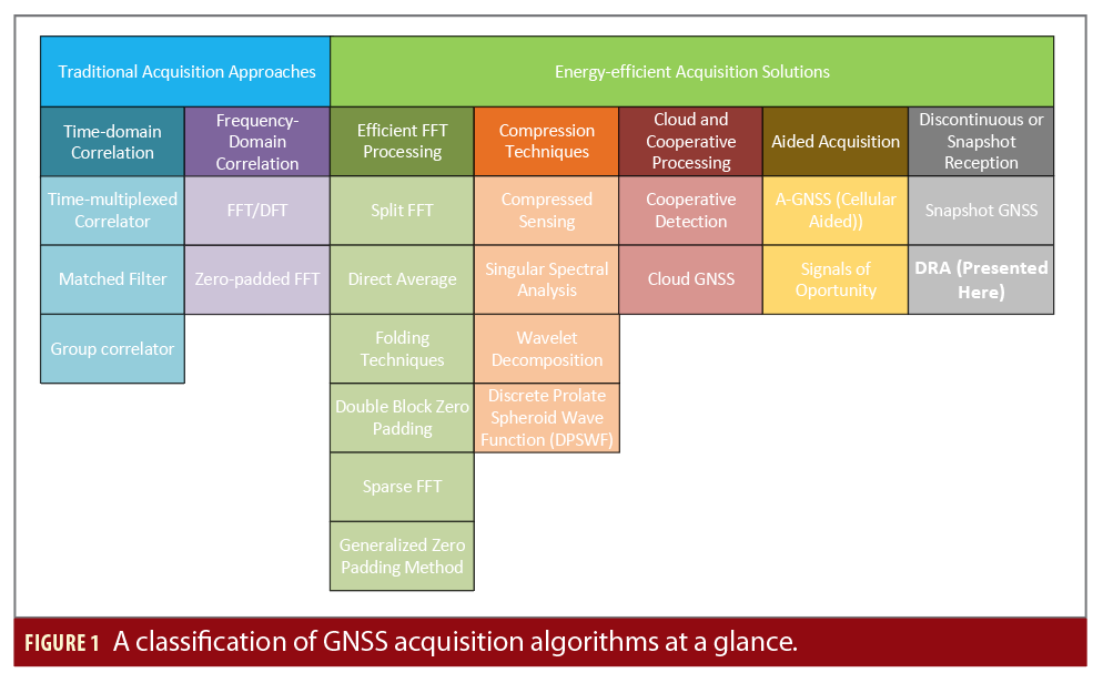
Figure 1 gives top-level classification of various GNSS acquisition algorithms from the current literature. Traditional GNSS acquisition approaches are based on time-domain or frequency-domain correlations with full-length acquisition, and they are either based on hardware implementations, such as including application specific integrated coud & cooperative processing) or on software iions, i.e., software-defined receivers (SDR). Many current GNSS acquisition units use frequency-domain approaches such as those based on fast Fourier transform (FFT), discrete Fourier Transform (DFT), or zero-padded FFT.
The energy-efficient acquisition solutions can be classified into five main classes, as shown in Figure 1.
The fourth class, methods relying on external (aiding) data, such as data coming from cellular networks (i.e., A-GNSS), or signals of opportunity such as Wi-Fi, BLE, LoRa, NB-IoT and so on, fall into the category of hybrid solutions, not standalone GNSS solutions and therefore lie outside the scope of this article.
In the fifth class, methods relying on discontinuous transmission or snapshot receivers, a case study using DRA is proposed and analyzed later in this article. Snapshot processing in general consists of sampling the GNSS signal for a very short time (e.g., few milliseconds), and processing the recorded digital samples in a post-processing stage. Its high flexibility offers multiple configurations, where the whole processing can be either performed on the device or entirely outsourced to the cloud. This category of methods can offer innovative and energy-efficient solutions, although its real-world adoption is currently only beginning.
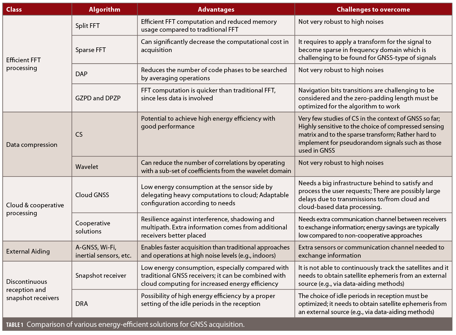
Table 1 summarizes our comparison of some of the above-mentioned approaches in terms of advantages, disadvantages, and outstanding challenges.
Complexity Considerations
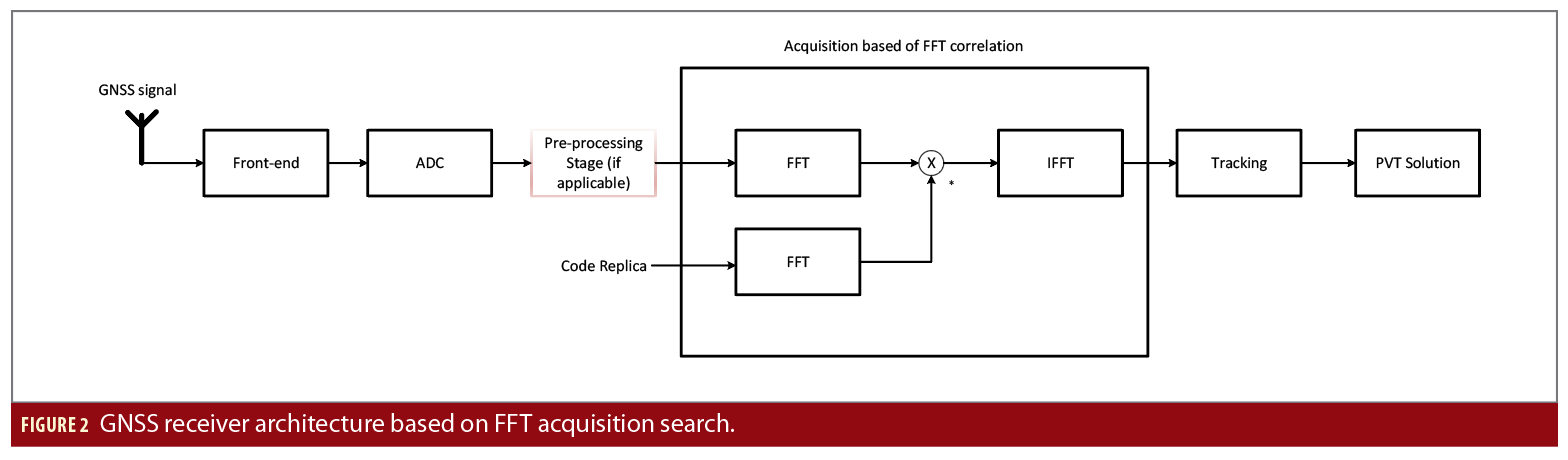
Figure 2 shows a block diagram of a generic GNSS receiver with a FFT-based acquisition stage. Here we address the complexity of the acquisition part by computing the number of operations involved in an FFT-based acquisition. The GNSS signal received from the antenna goes through the front-end processing, is down-converted to an intermediate frequency or directly to the baseband through the analog-to-digital converter (ADC) block. Then some additional pre-processing can take place, such as decimation, pre-correlation-based interference detection and mitigation. Finally the received signal enters the acquisition stage.
In this stage, correlations are performed with different code replicas, at different delays and Doppler shifts, based on the satellite codes; here an FFT-based acquisition is depicted. The tracking and position, velocity, time (PVT) computation blocks after the acquisition are also parts of a GNSS receiver, but not addressed in the complexity computations below, as typically most of the power reduction or energy-saving gains can come from the acquisition stage.
Typically, the complexity of an N-point FFT or IFFT approach where N is a power of 2 can be computed as:

where N is the FFT length, which is typically the next power of 2 higher or equal to Ns, with Ns being the number of samples per correlation interval. As seen in Figure 2, there are three FFT/IFFT such stages: one FFT applied to the incoming signal, one applied to the code replica, and an IFFT block applied to the product between the frequency-domain signal and the conjugate of the frequency-domain code.
If a signal with N-samples can be pre-processed in such a way to have K non-zero samples (i.e., K sparse) and N-K samples equal to zero in frequency domain, sparse FFT implementations of lower complexity than in Eq. (1) exist. Then the complexity can be decreased to:

or even to:

according to the type of sparse FFT implementation.
As an example of achievable computational reduction (and thus of increased energy efficiency), if one considers a T ms signal window with a sampling rate fs, there will be N=T·fs samples to process in the considered window. Assuming that a K-sparse signal can be achieved with an adequate transform (e.g., compressed sensing, etc.), this could coarsely translate to a compression factor of M=N/K, or, alternatively, a compression rate CR=(1-1/M)*100% (e.g., if N=1000, K=100, then M=10 and CR=90%). The the term K-sparse refers here to the number of non-zero samples of a signal (i.e., a 100-sparse signal with K=100 will have less zeros and mor non-zero terms than a 50-sparse signal, with K=50).
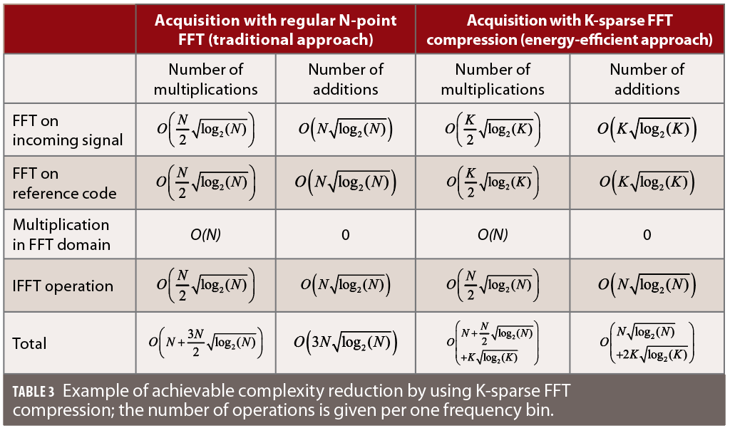
In terms of needed operations to perform the acquisition stage via a frequency-domain correlation, they are listed in Table 2. To approximately quantify the maximum achievable performance, the sparse FFT method (i.e., equation (3)) was considered. The complexity reduction comes from applying sparse FFT transforms on the incoming signal and reference code, which is used to perform the correlation between the incoming signal and the replica code. As the overall length of the considered signal window is N, the inverse FFT (IFFT) operations remain the same as for the traditional and energy-efficient FFT transforms.
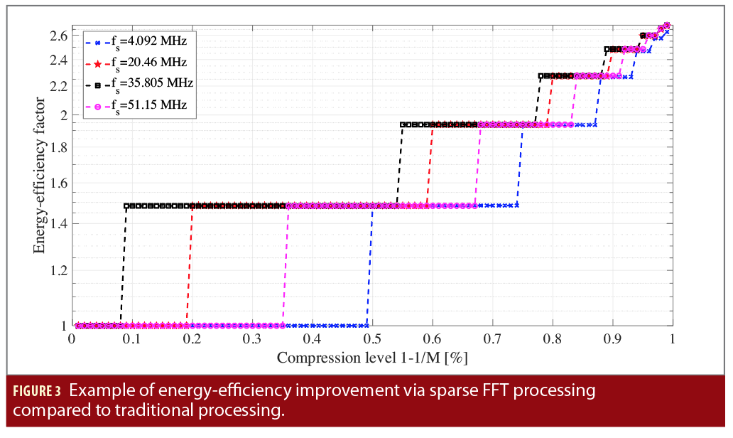
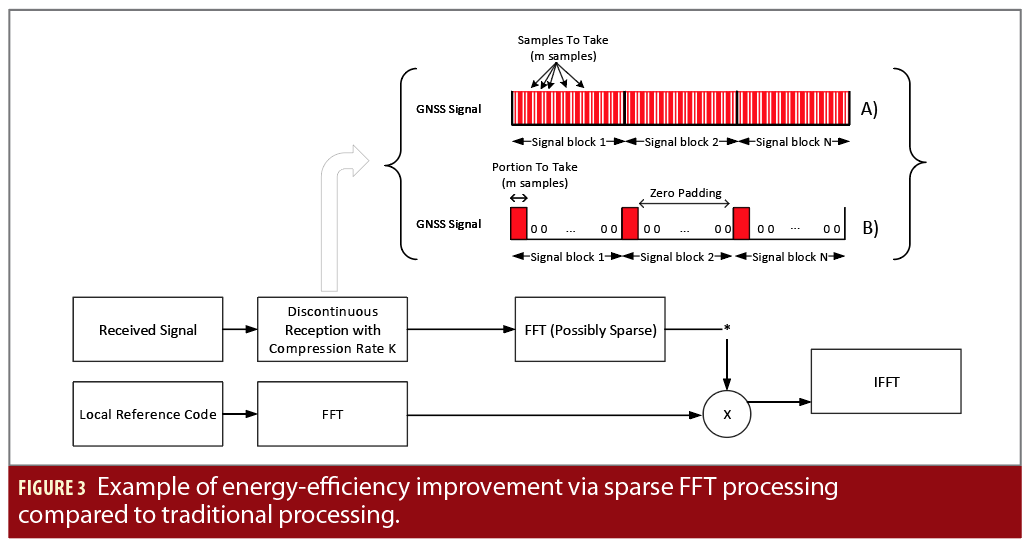
Considering that the efficiency bounds depicted in Table 2 are achievable when K is a power of 2, Figure 3 depicts a few illustrative examples for sampling frequencies fs between 4.092 MHz and 51.15 MHz. The stair-wise behavior comes from the fact that we consider a sparse implementation with K equal to a power of 2. It is to be noted that in literature there are now also efficient implementations of the FFT when the length is a power of 3, 5, etc. (these are called radix-N FFT), however these were not included in our example for clarity purposes.
In our example, K was computed based on a target compression level CR=(1-1/M)*100 (shown in percentage in the x axis of Figure 2), with K being the next power of 2 of N/M ratio. The energy-efficiency factor was defined here as the ratio between the number of operations with compressed acquisition with respect to the number of operations on a regular, no-compression FFT-based acquisition. The maximum energy- efficiency factor is close in our example to 2.7, and it is achieved for very high compression ratios (close to 99%), for which the performance to correctly acquire the satellites in view is clearly expected to deteriorate. Examples of achievable detection probabilities with various compression factors will be shown later.
Another observation based on the examples shown in Figure 2 is that high energy savings are hard to achieve even with a sparse FFT processing, and there is certainly place for novel and innovative solutions for higher energy-efficiency FFT processing. Moderate sampling frequency levels (e.g., 20.46 MHz and 35.80 MHz) are also able to reach higher energy efficiency than low and very-high sampling frequency, because of the condition of K factor to be a power of two.
Challenges in Compressed-Sensing
While CS approaches have been investigated to some extent in recent years in the context of GNSS, there are still many unsolved challenges in this field. This section briefly summarizes the CS concept and points out some of the challenges in applying CS with GNSS signals.
Any CS signal consists of three steps:
• measurement matrix generation;
• signal compression; and
• signal recovery.
The measurement matrix φ is the one in charge of mapping the data to the compressed domain and vice versa (from N dimension to a smaller dimension K, with N>K). The measurement matrix φ has dimensions KxN, and it can take different shapes. For example, it can be completely random or following a certain distribution/function such as discrete cosine transform (DCT), balanced Bernoulli (same number of +1 and -1), or based on a Kronecker (kron)-function approach. The choice of such measurement matrix is in fact the most challenging step when one deals with spread-spectrum types of signals. In our simulation-based analysis, the kron-type of measurement matrix gave the best results and is considered here.
To compress the GNSS signal x [34][35], with dimensions Nx1 one only needs to multiply x by the CS measurement matrix φ as

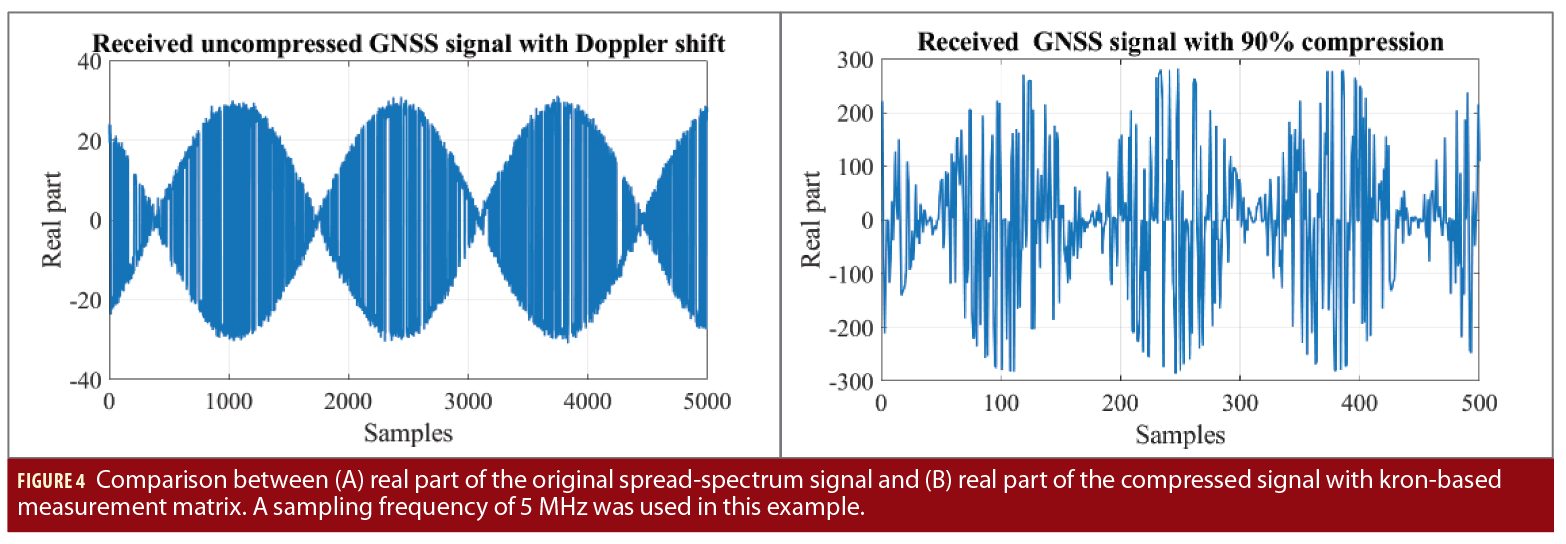
where y is the compressed signal with dimensions Kx1. Figure 4 gives an example of an original spread-spectrum signal (real part) and the same piece of signal with a 90% compression and a Bernoulli kron-based measurement (compression) matrix. We can see that the compressed signal shape is very different from the original. In the original we observe the modulated GNSS signal, while in the compressed domain it looks like random Gaussian noise. The advantage of such a processing is the fact that the length of the signal is reduced by a M=N/K factor (in this example 10 times), leading to a compression rate CR=(1-1/M)*100 of 90%.
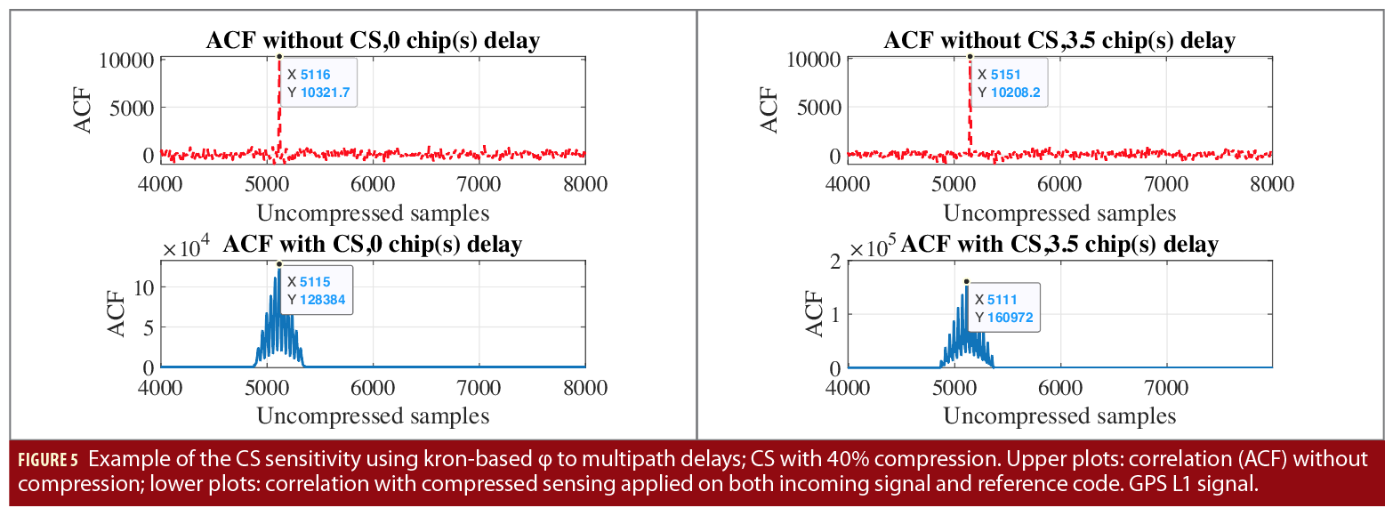
The last step in a CS processing is the signal decompression or recovery part. This can be done for example by applying known algorithms such as least squares, minimum mean square error, or gradient projection for sparse reconstruction. However, most of such algorithms are very sensitive to noise and multipath and they are challenging to operate with spread-spectrum type of signals. An example of such sensitivity to multipath channels is illustrated in Figure 5. Based on our observations, the presence of multipaths over the wireless channels introduce random delays in the correlation after CS operation, which are hard to be estimated and compensated at the receiver and thus represent a challenge in CS-based processing in GNSS.
As a brief conclusion of our analysis of CS approaches for GNSS, more research needs to be done to prove the viability of a CS approach in GNSS context.
Discontinuous-Reception Accquisition
Figure 6 shows a block diagram of the DRA. The reception of the incoming signal is done in intermittent blocks, either contiguous, in pieces of K samples at a time (as in the lower-plot B) of the block diagram in Figure 6) or non-contiguous [36] (e.g., by taking every m=N/K-th sample of the incoming signal, as shown in upper plot A of Figure 6). The non-contiguous DRA approach could be also seen as sort of decimation, followed by zero-padding, and this can introduce non-linearities such as aliasing and distortions and thus a compromise between the number of samples to take and discard for further analysis has to be found. The contiguous DRA is similar with the discontinuous reception (DRX) principle in wireless cellular communications.
The number of non-zero samples K can be adjusted in such a way to reach the desired compression rate CR (i.e., CR=(1-K/N)*100). The acquisition unit complexity can be thus decreased, for example by applying partial correlations with a code matrix saved in the receiver memory or by zero-padded FFT transform.
Simulation-based results. In a first step, the DRA algorithm has been tested with a MATLAB-based GNSS simulator, comprised of a GPS C/A transmitter, an additive Gaussian white noise (AWGN) channel, and a GPS acquisition unit based on frequency-domain correlation. A sampling frequency of 5 MHz was used, and acquisition results are shown for 1ms coherent integration and 5ms non-coherent integration.
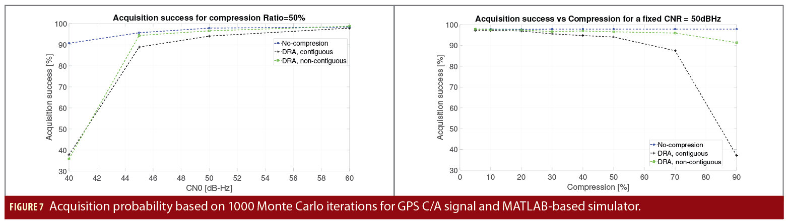
The simulation-based results are shown in Figure 7, based on 1000 Monte Carlo runs. In the simulations, GPS L1 C/A simulated signals were used with a sampling frequency Fs of 5 MSamples/s. The detection probability was computed as the probability to acquire the correct satellite with a delay error less than 0.5 chips and a Doppler error less than 250 Hz.
The figure shows that the non-contiguous DRA acquisition gives slightly better results than the contiguous DRA acquisition. The differences are small depending on the level of noise or compression ratios. As seen in Figure 7a, a compression factor of 2 (i.e., 50% compression rate) would deteriorate the carrier-to-noise ratio (C/N0) results with about 3dB especially at low C/N0, which points out to the tradeoff between performance and energy efficiency (here reflected in the amount of computations to perform the acquisition).
Mapping the results shown in Figure 2 with the provided in Figure 7, it is clear that the energy efficiency gain we can achieve is lower than the loss in detection performance (i.e., we are not able to reduce the energy consumption by half by compressing the signal by half). This result also illustrates the fact that high energy efficiency with reasonable performance loss is a challenging task to be achieved.
Figure 7b shows that the performance deterioration with 70% compression rate is much steeper with contiguous DRA than with non-contiguous DRA. About 10% of acquisition probability is lost with contiguous DRA at 70% compression rate while less than 5% is lost with non-contiguous at a C/N0=50 dB-Hz, but the acquisition performance deteriorates fast for higher compression rates, especially for contiguous DRA.
Measurement-based results. The DRA concept has also been tested with two set of recorded GPS C/A measurements: one dataset recorded at Universitat Autonoma de Barcelona (UAB), Spain, in 2013 (dataset 1) and another dataset (dataset 2) recorded at Tampere University (TAU), Finland in 2019. Dataset 1 was based on a low-cost recording approach using a SiGe GN3S receiver device and a patch antenna. Dataset 2 was based on a slightly more sophisticated approach, by using an USRP and a GPS roof antenna. The sampling frequency in dataset 1 was 5MHz, while sampling frequency in dataset 2 was taken at 50MHz. Both approaches used a computer as host device to control either the SiGe or the USRP receivers. The SiGe/USRP acted as a front-end and down-converted the RF signals to baseband, digitized them and sent the real/complex IQ-data to the host computer. With SiGe device the data was recorded as real data with 8-bits quantization. With the USRP (dataset 2), the data was recorded as complex-valued data with 16-bits quantization.
On the receiver side, the same coherent and non-coherent integration time as in the previous simulations were used (i.e., 1 ms coherent and 5 ms non-coherent integration times). As there is no ground-truth in the data collected from roof antennas, the reference was taken as being the signal without compression and the comparison metric was the match between the DRA algorithm (i.e., data with compression) and the non-compressed acquisition.
A match was declared if, simultaneously, three conditions were fulfilled:
• acquisition metric was higher than the acquisition threshold;
• the estimated code delays were within 0.5 chips apart from each other (in DRA and acquisition without compression) in absolute value, and
• the estimated Doppler shifts were within 250 Hz from each other, in absolute value.
The match values proved to jump from 100% to 0% when a certain compression rate was reached.
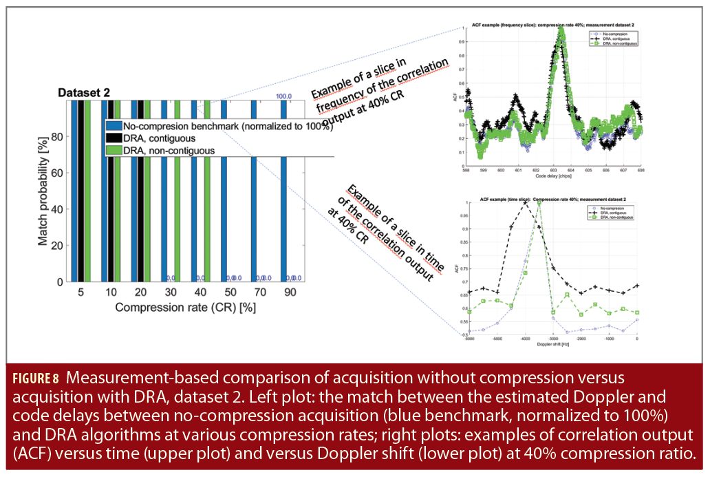
An example based on dataset 2 is shown in Figure 8. The right-hand plots illustrate why there is 0% match probability of the contiguous DRA with respect to the no-compression acquisition at 40% compression rate. Basically the mismatch comes from Doppler estimates, as can be seen in the lower right-side plot of Figure 8. Doppler estimation in contiguous DRA is far from the considered true Doppler estimation. Similarly, we can observe why we have 100% match of the non-contiguous DRA. Both estimated delays and estimated Doppler shifts are close to each other with respect to the no-compression acquisition estimates for the illustrated compression rate of 40%.
The compression rates at which the mismatch between the no-compression acquisition and DRA acquisition starts are shown in Table 3. The threshold percentages here are also in tune with what we observed from the left-side plot of Figure 7 at 40dBHz and 50 dB-Hz. The measurement-based C/N0 was estimated based on a well-known narrowband-wideband power ratio estimator. As the ground truth is not available, the thresholds in Table 3 are slightly different from what we observed in the right-plot of Figure 7, but this is because in Table 3 we are able to only compare the match between no-compression acquisition and DRA acquisition, but not to the absolute acquisition probability values.
Conclusions
We have investigated the expected complexity of various FFT-based approaches and discussed a few of the current shortcomings of compressed-sensing algorithms. We have also studied two implementations of higher energy-efficiency acquisition, namely a contiguous and a non-contiguous one, of a discontinuous reception algorithm.
It has been shown that moderate gains in energy efficiency are typically achievable at the expense of some acquisition performance loss and that non-contiguous-blocks discontinuous reception results in slightly better acquisition performance than contiguous-blocks discontinuous reception, thanks to exploiting better the variability of the pseudorandom code and of the channel effects. Achieving simultaneously very high sensitivity (i.e., good acquisition performance) and low power/high energy efficiency remains still a challenging task, and further research work on techniques with better trade-off between low power and high sensitivity is needed for future GNSS receivers.
In addition, the impact of fading multipath channels as well as of the interferences (e.g., jamming, spoofing, etc.) of such increased energy-efficiency acquisition algorithms is still to be studied.
Acknowledgments
We acknowledge the support to work by the Academy of Finland (project ULTRA, #328226 and #328214), by the doctoral school the Faculty of Information Technology and Communication Sciences of Tampere University, and by the ICREA Academia Program.
Authors

Ruben Morales-Ferre received an M.Sc. in telecommunication engineering from Universitat Autonoma de Barcelona and is pursuing a double Ph.D. degree in information and electrical engineering at the Dept. of Telecommunication, UniversitatAutonoma de Barcelona.

Gonzalo Seco-Granados received a Ph.D. in telecommunications engineering from the Universitat Politecnica de Catalunya and an M.B.A. from the IESE Business School, Spain. He is currently professor in the Dept. of Telecommunication, UniversitatAutonoma de Barcelona.

Elena Simona Lohan is a professor of electrical engineering at Tampere University, Finland, where she obtained her Ph.D. in telecommunications.


